| |
| | |
|
An operating model is the abstract representation of how an System operates
across process.
Any system is a complex system consisting of several different interlinked
logical components.
An operating model breaks this complexity into its logical components in order
to deliver better value.
Some examples of operational models are SCOOT, SCAT and OPAC which are
described below.
The Split Cycle Offset Optimization Technique (SCOOT) is an urban traffic
control system developed by the Transport Research Laboratory (TRL) in
collaboration with the UK traffic systems industry.
It is an adaptive system which responds automatically to traffic fluctuations.
Prime objective of this is to minimize the sum of the average queues in the
area.
It is an elastic coordination plan that can be stretched or shrunk to match the
latest traffic situation.
Continuously measures traffic volumes on all approaches of intersections in the
network and changes the signal timings to minimize a Performance Index (PI)
which is a composite measure of delay, queue length and stops in the network.
Each SCOOT cell is able to control up to 60 junctions.
Handling input data up to 256 vehicle counting detectors on street.
Detectors are usually positioned 14 m behind the stop line.
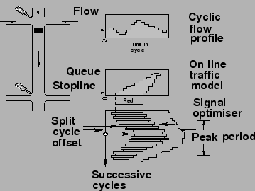
- Cycle Flow Profile’s (CFP) measure in real time
- Update an on-line model of queues continuously
- Incremental optimization of signal settings
- Cyclic Flow Profiles (CFP)
CFP is a measure of the average one-way flow of vehicles passed at any point on
the road during each part of the cycle time of the upstream signal.
It records the platoon of vehicles successively within a cycle time during peak
flow.
It updated in every 4 seconds.
CFP’s can be measured easily by hand.
Shape of the CFP has to be calculated for each one-way flow along all streets
in the area.
Accuracy of calculation depends on the accuracy of the data on average Flows,
saturation flows, and cruise times.
- Queue Estimation
It is necessary to predict new signal timing due to the queues after alteration
according to the situation after knowing CFP, the computer can be programmed to
estimate no of vehicles which will reach the downstream signals during red
phase.
So size of the queue and duration to clear the queue can be calculated.
In this calculation it is assumed that the traffic platoons travel at a known
cruising speed with some dispersion.
Queues discharge during the green time at a saturation flow rate that is known
and constant for each signal stop line.
- Incremental Optimization
Incremental Optimization is done to measure the coordination plan that it is
able to respond to new traffic situations in a series of frequent, but small,
increments.
It is necessary because research shows that prediction of traffic flow is very
difficult for next few minutes.
SCOOT split optimizer calculates whether it is good to advance or retard the
scheduled change by up to 4 s, or to leave it unaltered.
It is achieved by split optimization, offset optimization, cycle time.
- Split Optimizer
Works at every change of stage by analyzing the current red and green timings
to determine whether the stage change time should be advanced, retarded or
remain the same.
Works in increments of 1 to 4 seconds.
- Cycle Time Optimizer
It operates on a region basis once every five minutes, or every two and a half
minutes.
Identifies the ``critical node'' within the region and will attempt to adjust
the cycle time to maintain this node with 90% link saturation on each stage.
It can increase or decrease the cycle time in 4, 8 or 16 second increments
according to the current requirement of the traffic flow.
- Offset Optimizer
It works once per cycle for each node.
It operates by analyzing the current situation at each node using the cyclic
flow profiles predicted for each of the links with upstream or downstream
nodes.
It assesses whether the existing action time should be advanced, retarded or
remains the same in 4 second increments.
Fig. 1 is showing the key elements of the SCOOT ATC
system which we described in above points.
Figure 1:
Key elements of the SCOOT ATC system (Source: Dennis I. Robertson and
R. David Bretherton 1991)
 |
Scoot system consists of a number of SCOOT cells or computers, each cell can
control up to 60 junctions and handling input data from up to 256 vehicle
counting detectors on street.
SCOOT detectors are placed at 14 m from the stop-line, from the approach to the
junction as possible.
Fig. 2 clearly shows the working principle of SCOOT
where the detectors placed upstream sense the occupancy and the information is
transmitted to the central computer.
SCOOT traffic model and optimizers use this information to calculate signal
timings to achieve the best overall compromise for coordination along all links
in the SCOOT area.
The main aim of the SCOOT traffic signal control system is to react to changes
in observed average traffic demands by making frequent, but small, adjustments
to the signal cycle time, green allocation, and offset of every controlled
intersection.
For each coordinated area, the system evaluates every 5 minutes, or 2.5 minutes
if appropriate, whether the common cycle time in operation at all intersections
within the area should be changed to keep the degree of saturation of the most
heavily loaded intersection at or below 90%.
In normal operation SCOOT estimates whether any advantage is to be gained by
altering the timings.
Fig. 2 is showing the working principle of SCOOT.
Figure 2:
Working Principle of SCOOT (Source: www.scoot-utc.com)
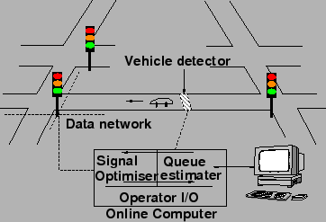 |
From above fig we can have an idea that vehicle will be detected with the help
of vehicle detector.
The collected data will be send to intersection controller after that it will
be send to the central controller with the help of communication network.
There it will be use to estimate the signal timing according to the actual
traffic flow needs.
Then the central controller will send the signal timing to the intersection
controller to implement.
- Variable Message Signs
Scoot display message signs to convey the guidance to the driver which is very
helpful for the drive.
- Diversions
This feature is provided to deal with any emergency situation for example if
any problem is found out in any lane which is found out with the help of Fault
Identification & Management unit then traffic will be diverted from that lane
to another lane.
- Emergency Green Wave Routes
This feature is provided to deal with any hazardous situation.
- Fixed Time Plan
This plan is applied when any unit of ATCS stopped working so till the time
that unit starts functioning.
- Inability to handle closely spaced signals due to its particular
detection configuration requirements, its require some time to detect vehicle.
- Interface is difficult to handle, as this is highly technical so
difficult to understand and handle.
- Traffic terminologies are different from those used in India.
- Primarily designed to react to long-term, slow variations in traffic
demand, and not to short-term random fluctuations.
|
|
| | |
|
|
|