| |
| | |
|
The values derived from the delay calculations represent the average control
delay experienced by all vehicles that arrive in the analysis period, including
delays incurred beyond the analysis period when the lane group is
oversaturated.
The average control delay per vehicle for a given lane group is given by
Equation,
where, d = control delay per vehicle (s/veh);  = uniform control delay
assuming uniform arrivals (s/veh); PF = uniform delay progression adjustment
factor, = uniform control delay
assuming uniform arrivals (s/veh); PF = uniform delay progression adjustment
factor,  = incremental delay to account for effect of random arrivals and = incremental delay to account for effect of random arrivals and
 = initial queue delay, which accounts for delay to all vehicles in
analysis period
Good signal progression will result in a high proportion of vehicles arriving
on the uniform delay Green and vice-versa.
Progression primarily affects uniform delay, and for this reason, the
adjustment is applied only to d1.
The value of PF may be determined using Equation, = initial queue delay, which accounts for delay to all vehicles in
analysis period
Good signal progression will result in a high proportion of vehicles arriving
on the uniform delay Green and vice-versa.
Progression primarily affects uniform delay, and for this reason, the
adjustment is applied only to d1.
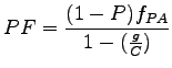
The value of PF may be determined using Equation,
 |
(1) |
where, PF = progression adjustment factor, P = proportion of vehicles arriving
on green, g/C = proportion of green time available,  = supplemental
adjustment factor for platoon arriving during green.
The approximate ranges of RP are related to arrival type as shown below. = supplemental
adjustment factor for platoon arriving during green.
The approximate ranges of RP are related to arrival type as shown below.
Table 1:
Relation between arrival type (AT) and platoon ratio
| AT |
Ration |
Default  |
Progression quality |
| 1 |
 |
0.333 |
very poor |
| 2 |
0.50-0.85 |
0.667 |
Unfavorable |
| 3 |
0.85-1.15 |
1.000 |
Random arrivals |
| 4 |
1.15-1.50 |
1.333 |
Favorable |
| 5 |
1.50-2.00 |
1.667 |
Highly favorable |
| 6 |
2.00 |
2.000 |
Exceptional |
PF may be calculated from measured values of P using the given values of
 or the following table can be used to determine PF as a function of
the arrival type. or the following table can be used to determine PF as a function of
the arrival type.
Table 2:
Progression adjustment factor for uniform delay calculation
| Green Ratio |
Arrival Type (AT) |
| (g/C) |
AT1 |
AT2 |
AT3 |
AT4 |
AT5 |
AT6 |
| 0.2 |
1.167 |
1.007 |
1 |
1 |
0.833 |
0.75 |
| 0.3 |
1.286 |
1.063 |
1 |
0.986 |
0.714 |
0.571 |
| 0.4 |
1.445 |
1.136 |
1 |
0.895 |
0.555 |
0.333 |
| 0.5 |
1.667 |
1.24 |
1 |
0.767 |
0.333 |
0 |
| 0.6 |
2.001 |
1.395 |
1 |
0.576 |
0 |
0 |
| 0.7 |
2.556 |
1.653 |
1 |
0.256 |
0 |
0 |
|
1 |
0.93 |
1 |
1.15 |
1 |
1 |
| Default, |
0.333 |
0.667 |
1 |
1.333 |
1.667 |
2 |
It is based on assuming uniform arrival, uniform flow rate & no initial queue.
The formula for uniform delay is,
![$\displaystyle d_1 = \frac{0.5C(1-\frac{g}{C})^2}{1-[min(1,X)\frac{g}{C}]}$](img10.png) |
(2) |
where, = uniform control delay assuming uniform arrivals (s/veh), C =
cycle length (s); cycle length used in pre-timed signal control, g = effective
green time for lane group, X = v/c ratio or degree of saturation for lane
group.
The equation below is used to estimate the incremental delay due to nonuniform
arrivals and temporary cycle failures (random delay.
The equation assumes that there is no unmet demand that causes initial queues
at the start of the analysis period (T).
![$\displaystyle d_2=900~T\left[(X-1)+\sqrt{(X-1)^2+\frac{8klX}{cT}}\right]$](img11.png) |
(3) |
where, = incremental delay queues, T = duration of analysis period (h); k
= incremental delay factor that is dependent on controller settings, I =
upstream filtering/metering adjustment factor; c = lane group capacity (veh/h),
X = lane group v/c ratio or degree of saturation, and K can be found out from
the following table.
Table 3:
k-values to account for controller type
| Unit |
Degree of Saturation (X) |
| Extension (s) |
|
0.6 |
0.7 |
0.8 |
0.9 |
 |
 |
0.04 |
0.13 |
0.22 |
0.32 |
0.41 |
0.5 |
| 2.5 |
0.08 |
0.16 |
0.25 |
0.33 |
0.42 |
0.5 |
| 3 |
0.11 |
0.19 |
0.27 |
0.34 |
0.42 |
0.5 |
| 3.5 |
0.13 |
0.2 |
0.28 |
0.35 |
0.43 |
0.5 |
| 4 |
0.15 |
0.22 |
0.29 |
0.36 |
0.43 |
0.5 |
| 4.5 |
0.19 |
0.25 |
0.31 |
0.38 |
0.44 |
0.5 |
 |
0.23 |
0.28 |
0.34 |
0.39 |
0.45 |
0.5 |
| Pre-timed |
0.5 |
0.5 |
0.5 |
0.5 |
0.5 |
0.5 |
The delay obtained has to be aggregated, first for each approach and then for
the intersection
The weighted average of control delay is given as:
where,  = delay per vehicle for each movement (s/veh), = delay per vehicle for each movement (s/veh),  = delay for
Approach A (s/veh), and = delay for
Approach A (s/veh), and  = adjusted flow for Approach A (veh/h). = adjusted flow for Approach A (veh/h).
Intersection LOS is directly related to the average control delay per vehicle.
Any v/c ratio greater than 1.0 is an indication of actual or potential
breakdown.
In such cases, multi-period analyses are advised.
These analyses encompass all periods in which queue carryover due to
oversaturation occurs.
A critical v/c ratio greater than 1.0 indicates that the overall signal and
geometric design provides inadequate capacity for the given flows.
In some cases, delay will be high even when v/c ratios are low.
Table 4:
LOS criteria for signalized intersection in term of control delay per
vehicle (s/veh)
| LOS |
Delay |
| A |
 |
| B |
10-20 |
| C |
20-35 |
| D |
35-55 |
| E |
55-80 |
| F |
 80 80 |
The predicted delay is highly sensitive to signal control characteristics and
the quality of progression.
The predicted delay is sensitive to the estimated saturation flow only
when demand approaches or exceeds 90 percent of the capacity for a lane group or
an intersection approach.
The following graph shows the sensitivity of the predicted control delay per
vehicle to demand to capacity ratio, g/c, cycle length and length of analysis
period.
Figure 1:
sensitivity of delay to demand to capacity ratio
|
|
Assumptions are :
Cycle length = 100s, g/c = 0.5, T =1h, k = 0.5, l= 1, s = 1800 veh/hr
Figure 2:
sensitivity of delay Vs g/c ratio
|
|
Figure 3:
sensitivity of delay Vs cycle length
|
|
|
|
| | |
|
|
|
![\includegraphics[height = 5cm]{qfdemandcapacitygraph1}](img22.png)
![\includegraphics[height = 5cm]{qfdelaygraph2}](img23.png)
![\includegraphics[height = 5cm]{qfdelaycyclelengthgraph3}](img24.png)