| |
| | |
|
The next step in the determination of the LOS is the computation of the peak
hour factor.
The fifteen minute passenger-car equivalent flow rate (pc/h/ln), is determined
by using following formula:
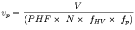 |
(1) |
where,  is the 15-min passenger-car equivalent flow rate (pc/h/ln), is the 15-min passenger-car equivalent flow rate (pc/h/ln),
 is the hourly volume (veh/h), is the hourly volume (veh/h),
 is the peak-hour factor, is the peak-hour factor,
 is the number of lanes, is the number of lanes,
 is the heavy-vehicle adjustment factor, and is the heavy-vehicle adjustment factor, and
 is the driver population factor.
PHF represents the variation in traffic flow within an hour.
Observations of traffic flow consistently indicate that the flow rates found in
the peak 15-min period within an hour are not sustained throughout the entire
hour.
The PHFs for multilane highways have been observed to be in the range of 0.75
to 0.95.
Lower values are typical of rural or off-peak conditions, whereas higher
factors are typical of urban and suburban peak-hour conditions.
Where local data are not available, 0.88 is a reasonable estimate of the PHF
for rural multilane highways and 0.92 for suburban facilities.
Besides that, the presence of heavy vehicles in the traffic stream decreases
the FFS because base conditions allow a traffic stream of passenger cars only.
Therefore, traffic volumes must be adjusted to reflect an equivalent flow rate
expressed in passenger cars per hour per lane (pc/h/ln).
This is accomplished by applying the heavy-vehicle factor ().
Once values for is the driver population factor.
PHF represents the variation in traffic flow within an hour.
Observations of traffic flow consistently indicate that the flow rates found in
the peak 15-min period within an hour are not sustained throughout the entire
hour.
The PHFs for multilane highways have been observed to be in the range of 0.75
to 0.95.
Lower values are typical of rural or off-peak conditions, whereas higher
factors are typical of urban and suburban peak-hour conditions.
Where local data are not available, 0.88 is a reasonable estimate of the PHF
for rural multilane highways and 0.92 for suburban facilities.
Besides that, the presence of heavy vehicles in the traffic stream decreases
the FFS because base conditions allow a traffic stream of passenger cars only.
Therefore, traffic volumes must be adjusted to reflect an equivalent flow rate
expressed in passenger cars per hour per lane (pc/h/ln).
This is accomplished by applying the heavy-vehicle factor ().
Once values for  and and  have been determined, the adjustment factors
for heavy vehicles are applied as follows: have been determined, the adjustment factors
for heavy vehicles are applied as follows:
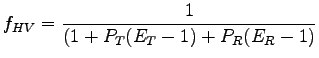 |
(2) |
where,
and are the equivalents for trucks and buses and for recreational
vehicles (RVs), respectively,
 and and  are the proportion of trucks and buses, and RVs, respectively,
in the traffic stream (expressed as a decimal fraction), are the proportion of trucks and buses, and RVs, respectively,
in the traffic stream (expressed as a decimal fraction),
 is the adjustment factor for heavy vehicles.
Adjustment for the presence of heavy vehicles in traffic stream applies for
three types of vehicles: trucks, buses and recreational vehicles (RVs).
Trucks cover a wide range of vehicles, from lightly loaded vans and panel
trucks to the most heavily loaded coal, timber, and gravel haulers.
An individual truck's operational characteristics vary based on the weight of
its load and its engine performance.
RVs also include a broad range: campers, self-propelled and towed; motor homes;
and passenger cars or small trucks towing a variety of recreational equipment,
such as boats, snowmobiles, and motorcycle trailers.
There is no evidence to indicate any distinct differences between buses and
trucks on multilane highways, and thus the total population is combined. is the adjustment factor for heavy vehicles.
Adjustment for the presence of heavy vehicles in traffic stream applies for
three types of vehicles: trucks, buses and recreational vehicles (RVs).
Trucks cover a wide range of vehicles, from lightly loaded vans and panel
trucks to the most heavily loaded coal, timber, and gravel haulers.
An individual truck's operational characteristics vary based on the weight of
its load and its engine performance.
RVs also include a broad range: campers, self-propelled and towed; motor homes;
and passenger cars or small trucks towing a variety of recreational equipment,
such as boats, snowmobiles, and motorcycle trailers.
There is no evidence to indicate any distinct differences between buses and
trucks on multilane highways, and thus the total population is combined.
Table 1:
Passenger-car equivalent on extended general highway segments(Source:
HCM, 2000)
| Factor |
Type of Terrain |
| |
Level |
Rolling |
Mountainous |
| ET (Trucks and Buses) |
1.5 |
2.5 |
4.5 |
| ER (RVs) |
1.2 |
2.0 |
4.0 |
The level of service on a multilane highway can be determined directly from
Fig. ![[*]](file:/usr/local/share/lib/latex2html/icons/crossref.png) or Table-2 based on the free-flow speed (FFS) and the
service flow rate (vp) in pc/h/ln.
The procedure as follows: or Table-2 based on the free-flow speed (FFS) and the
service flow rate (vp) in pc/h/ln.
The procedure as follows:
- Define a segment on the highway as appropriate.
The following conditions help to define the segmenting of the highway,
- Change in median treatment
- Change in grade of 2% or more or a constant upgrade over 1220 m
- Change in the number of travel lanes
- The presence of a traffic signal
- A significant change in the density of access points
- Different speed limits
- The presence of bottleneck condition
In general, the minimum length of study section should be 760 m, and the limits
should be no closer than 0.4 km from a signalized intersection.
- On the basis of the measured or estimated free-flow speed on a highway
segment, an appropriate speed-flow curve of the same as the typical curves is
drawn.
- Locate the point on the horizontal axis corresponding to the appropriate
flow rate (vp) in pc/hr/ln and draw a vertical line.
- Read up the FFS curve identified in step 2 and determine the average
travel speed at the point of intersection.
- Determine the level of service on the basis of density region in which
this point is located.
Density of flow can be computed as
 |
(3) |
where,
 is the density (pc/km/ln),
is the flow rate (pc/h/ln), and is the density (pc/km/ln),
is the flow rate (pc/h/ln), and
 is the average passenger-car travel speed (km/h).
The level of service can also be determined by comparing the computed density
with the density ranges shown in table given by HCM.
To use the procedures for a design, a forecast of future traffic volumes has to
be made and the general geometric and traffic control conditions, such as speed
limits, must be estimated.
With these data and a threshold level of service, an estimate of the number of
lanes required for each direction of travel can be determined. is the average passenger-car travel speed (km/h).
The level of service can also be determined by comparing the computed density
with the density ranges shown in table given by HCM.
To use the procedures for a design, a forecast of future traffic volumes has to
be made and the general geometric and traffic control conditions, such as speed
limits, must be estimated.
With these data and a threshold level of service, an estimate of the number of
lanes required for each direction of travel can be determined.
|
|
| | |
|
|
|