| |
| | |
|
As already noted in the previous chapter that vehicle arrivals can be modelled
in two inter-related ways; namely modelling how many vehicle arrive in a given
interval of time, or modelling what is the time interval between the successive
arrival of vehicles.
Having discussed in detail the former approach in the previous chapter, the
first part of this chapter discuss how a discrete distribution can be used to
model the vehicle arrival.
Traditionally, Poisson distribution is used to model the random process, the
number of vehicles arriving a given time period.
The second part will discuss methodologies to generate random vehicle arrivals,
be it the generation of random headways or random number of vehicles in a given
duration.
The third part will elaborate various ways of evaluating the performance of a
distribution.
Suppose, if we plot the arrival of vehicles at a section as dot in a time axis,
it may look like Figure 1.
Figure 1:
Illustration of vehicle arrival modeling
 |
Let  , ,  , ... etc indicate the headways, then as mentioned earlier,
they take some real values.
Hence, these headways or inter arrival time can be modelled using some continuous
distribution.
Also, let , ... etc indicate the headways, then as mentioned earlier,
they take some real values.
Hence, these headways or inter arrival time can be modelled using some continuous
distribution.
Also, let  , ,  , ,  and and  are four equal time intervals, then the
number of vehicles arrived in each of these interval is an integer value.
For example, in Fig. 1, 3, 2, 3 and 1 vehicles arrived in
time interval , , and respectively.
Any discrete distribution that best fit the observed number of vehicle arrival
in a given time interval can be used.
Similarly, any continuous distribution that best fit the observed headways (or
inter-arrival time) can be used in modelling.
However, since these process are inter-related, the distributions that describe
these relations should also be inter-related for better explanation of the
phenomenon.
Interestingly, there exist distributions that meet the above requirements.
First, we will see the distribution to model the number of vehicles arrived in a
given duration of time.
Poisson distribution is commonly used to describe such a random process.
The probability density function of the Poisson distribution is given as: are four equal time intervals, then the
number of vehicles arrived in each of these interval is an integer value.
For example, in Fig. 1, 3, 2, 3 and 1 vehicles arrived in
time interval , , and respectively.
Any discrete distribution that best fit the observed number of vehicle arrival
in a given time interval can be used.
Similarly, any continuous distribution that best fit the observed headways (or
inter-arrival time) can be used in modelling.
However, since these process are inter-related, the distributions that describe
these relations should also be inter-related for better explanation of the
phenomenon.
Interestingly, there exist distributions that meet the above requirements.
First, we will see the distribution to model the number of vehicles arrived in a
given duration of time.
Poisson distribution is commonly used to describe such a random process.
The probability density function of the Poisson distribution is given as:
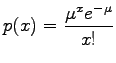 |
(1) |
where  is the probability for is the probability for  events will occur in the time interval, and events will occur in the time interval, and  is the expected
rate of occurrence of that event in that interval.
Some special cases of this distribution is given below. is the expected
rate of occurrence of that event in that interval.
Some special cases of this distribution is given below.
Since the events are discrete, the probability that certain number of
vehicles ( )
arriving in an interval can be computed as: )
arriving in an interval can be computed as:
Similarly, the probability that the number of vehicles arriving in the interval
is exactly in a range (between  and and  , both inclusive and , both inclusive and  ) is given as: ) is given as:
|
|
| | |
|
|
|


