| |
| | |
|
The hourly flow rate in a road section is 120 vph.
Use Poisson distribution to model this vehicle arrival.
The flow rate is given as ( ) = 120 vph = ) = 120 vph =
 = 2 vehicle per
minute.
Hence, the probability of zero vehicles arriving in one minute = 2 vehicle per
minute.
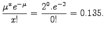
Hence, the probability of zero vehicles arriving in one minute  can be computed
as follows: can be computed
as follows:
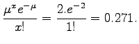
Similarly, the probability of one vehicles arriving in one minute  is given by, is given by,
Now, the probability that number of vehicles arriving is less than or equal to
zero is given as
Similarly, probability that the number of vehicles arriving is less than or equal
to 1 is given as:
Again, the probability that the number of vehicles arriving is between 2 to 4 is
given as:
Now, if the
 , then the number of intervals in an hour where there
is no vehicle arriving is , then the number of intervals in an hour where there
is no vehicle arriving is
The above calculations can be repeated for all the cases as tabulated in
Table 1.
Table 1:
Probability values of vehicle arrivals computed using Poisson distribution
 |
 |
 |
 |
| 0 |
0.135 |
0.135 |
8.120 |
| 1 |
0.271 |
0.406 |
16.240 |
| 2 |
0.271 |
0.677 |
16.240 |
| 3 |
0.180 |
0.857 |
10.827 |
| 4 |
0.090 |
0.947 |
5.413 |
| 5 |
0.036 |
0.983 |
2.165 |
| 6 |
0.012 |
0.995 |
0.722 |
| 7 |
0.003 |
0.999 |
0.206 |
| 8 |
0.001 |
1.000 |
0.052 |
| 9 |
0.000 |
1.000 |
0.011 |
| 10 |
0.000 |
1.000 |
0.011 |
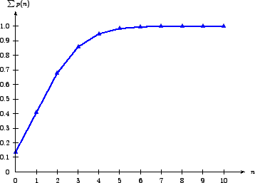
The shape of this distribution can be seen from Figure 1
and the corresponding cumulative distribution is shown in
Figure 2.
Figure 1:
Probability values of vehicle arrivals computed using Poisson distribution
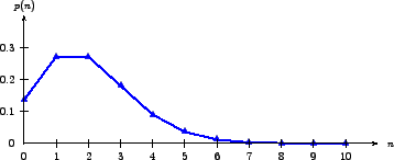 |
Figure 2:
Cumulative probability values of vehicle arrivals computed using Poisson distribution
 |
|
|
| | |
|
|
|