| |
| | |
|
For simulation purposes, it may be required to generate number of vehicles
arrived in a given interval so that it follows typical vehicle arrival.
This is the reverse of computing the probabilities as seen above.
The following steps give the procedure:
- Input: mean arrival rate
 in an interval in an interval 
- Compute
 and and

- Generate a random number
 such that such that

- Find
 such that such that
 and and
- Set
 , where , where  is the number of vehicles arrived in is the number of vehicles arrived in  interval.
The steps 3 to 5 can be repeated for required number of intervals.
Generate vehicles for ten minutes if the flow rate is 120 vph.
The first two steps of this problem is same as the example problem solved
earlier and the resulted from the table is used.
For the first interval, the random number () generated is 0.201 which is greater
than  but less than but less than  .
Hence, the number of vehicles generated in this interval is one ( .
Hence, the number of vehicles generated in this interval is one ( ).
Similarly, for the subsequent intervals.
It can also be computed that at the end of 10th interval (one minute), total 23 vehicle
are generated.
Note: This amounts to 2.3 vehicles per minute which is higher than given flow rate.
However, this discrepancy is because of the small number of intervals conducted.
If this is continued for one hour, then this average will be about 1.78 and if
continued for then this average will be close to 2.02. ).
Similarly, for the subsequent intervals.
It can also be computed that at the end of 10th interval (one minute), total 23 vehicle
are generated.
Note: This amounts to 2.3 vehicles per minute which is higher than given flow rate.
However, this discrepancy is because of the small number of intervals conducted.
If this is continued for one hour, then this average will be about 1.78 and if
continued for then this average will be close to 2.02.
Table 1:
Vehicles generated using Poisson distribution
| No |
X |
n |
| 1 |
0.201 |
1 |
| 2 |
0.714 |
3 |
| 3 |
0.565 |
2 |
| 4 |
0.257 |
1 |
| 5 |
0.228 |
1 |
| 6 |
0.926 |
4 |
| 7 |
0.634 |
2 |
| 8 |
0.959 |
5 |
| 9 |
0.188 |
1 |
| 10 |
0.832 |
3 |
| |
Total |
23 |
One can generate random variate following negative exponential distribution rather simply due to availability of closed form solutions.
The method for generating exponential variates is based on inverse transform sampling:
has an exponential distribution, where  , called as quantile function, is defined as , called as quantile function, is defined as
Note that if is uniform, then  is also uniform and is also uniform and
 .
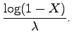
Hence, one can generate exponential variates as follows: .
Hence, one can generate exponential variates as follows:
where, is a random number between 0 and 1, is the mean headway, and the resultant headways generated () will follow exponential distribution.
Simulate the headways for 10 vehicles if the flow rate is 120 vph.
Since the given flow rate is 120 vph, then the mean headway () is 30
seconds.
Generate a random number between 0 and 1 and let this be 0.62.
Hence, by the above equation,
 .
Similarly, headways can be generated.
The table below given the generation of 15 vehicles and it takes little over 10
minutes.
In other words, the table below gives the vehicles generated for 10 minutes.
Note:
The mean headway obtained from this 15 headways is about 43 seconds; much higher
than the given value of 30 seconds.
Of, course this is due to the lower sample size.
For example, if the generation is continued to 100 vehicles, then the mean
would be about 35 seconds, and if continued till 1000 vehicles, then the mean
would be about 30.8 seconds. .
Similarly, headways can be generated.
The table below given the generation of 15 vehicles and it takes little over 10
minutes.
In other words, the table below gives the vehicles generated for 10 minutes.
Note:
The mean headway obtained from this 15 headways is about 43 seconds; much higher
than the given value of 30 seconds.
Of, course this is due to the lower sample size.
For example, if the generation is continued to 100 vehicles, then the mean
would be about 35 seconds, and if continued till 1000 vehicles, then the mean
would be about 30.8 seconds.
Table 2:
Headways generated using Exponential distribution
| No |
|
|
 |
| 1 |
0.62 |
14.57 |
14.57 |
| 2 |
0.17 |
53.70 |
68.27 |
| 3 |
0.27 |
39.14 |
107.41 |
| 4 |
0.01 |
157.36 |
264.77 |
| 5 |
0.26 |
40.01 |
304.78 |
| 6 |
0.47 |
22.72 |
327.5 |
| 7 |
0.96 |
1.38 |
328.88 |
| 8 |
0.24 |
42.76 |
371.64 |
| 9 |
0.59 |
15.94 |
387.58 |
| 10 |
0.45 |
24.05 |
411.63 |
| 11 |
0.26 |
40.82 |
452.45 |
| 12 |
0.11 |
67.39 |
519.84 |
| 13 |
0.10 |
69.33 |
589.17 |
| 14 |
0.73 |
9.63 |
598.8 |
| 15 |
0.31 |
34.74 |
633.54 |
The mathematical distribution such as negative exponential distribution, normal
distribution, etc needs to be evaluated to see how best these distributions
fits the observed data.
It can be evaluated by comparing some aggregate statistics as discussed below.
One of the easiest ways to compute the mean and standard deviation of the
observed data and compare with mean and standard deviation obtained from the
computed frequencies.
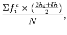
If  is the computed probability of the headway is the interval,
and is the computed probability of the headway is the interval,
and  is the total number of observations, then the computed frequency of the
interval is given as: is the total number of observations, then the computed frequency of the
interval is given as:
Then the mean of the computed frequencies ( ) is obtained as ) is obtained as
where  is the lower limit of the interval, and is the lower limit of the interval, and  is the
interval range.
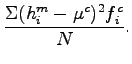
The standard deviation is the
interval range.
The standard deviation  can be obtained by can be obtained by
If the distribution fit closely, then the mean and the standard deviation of
the observed and fitted data will match.
However, it is possible, that two sample can have similar mean and standard
deviation, but, may differ widely in the individual interval.
Hence, this can be considered as a quick test for the comparison purposes.
For better comparison, Chi-square test which gives a better description of the
suitability of the distribution may be used.
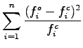
The Chi-square value ( ) can be computed using the following formula: ) can be computed using the following formula:
where  is the observed frequency, is the observed frequency,  is the computed (theoretical) frequency of
the interval, and is the number of intervals.
Obviously, a value close to zero implies a good fit of the data, while,
high value indicate poor fit.
For an objective comparison Chi-square tables are used.
A chi-square table gives values for various degree of freedom.
The degree of freedom (DOF) is given as is the computed (theoretical) frequency of
the interval, and is the number of intervals.
Obviously, a value close to zero implies a good fit of the data, while,
high value indicate poor fit.
For an objective comparison Chi-square tables are used.
A chi-square table gives values for various degree of freedom.
The degree of freedom (DOF) is given as
where n is the number of intervals, and p is the number of parameter defining the distribution.
Since negative exponential distribution is defined by mean headway alone, the value of
p is one, where as Pearson and Normal distribution has the value of p as
two, since they are defined by and  .
Chi-square value is obtained from various significant levels.
For example, a significance level of 0.05 implies that the likelihood that the observed frequencies following the theoretical distribution is
is 5%.
In other words, one could say with 95% confidence that the observed data follows the theoretical distribution under testing. .
Chi-square value is obtained from various significant levels.
For example, a significance level of 0.05 implies that the likelihood that the observed frequencies following the theoretical distribution is
is 5%.
In other words, one could say with 95% confidence that the observed data follows the theoretical distribution under testing.
|
|
| | |
|
|
|