The y -component of velocity profile can be obtained by differentiating stream function with respect to x and substituting the results from Eq. (5.9.4 & 5.9.6).

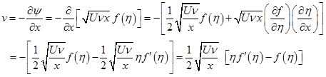(5.9.8)

Now, let us calculate each term of Eq. (5.9.1) from the velocity components obtained from Eqs (5.9.7 & 5.9.8).

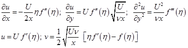(5.9.9)

Substitute each term of Eq. (5.9.9) in Eq. (5.9.1) and after simplification, the boundary layer equation reduces to Blasius equation expressed in terms of similarity variable.

(5.9.10)

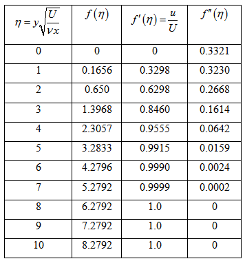
Table 5.9.1: Solution of Blasius laminar flat plate boundary layer in similarity variables

 

In certain cases, one can define for which Eq. (5.9.10) takes the following form;

(5.9.11)

The Blasius equation is a third-order non-linear ordinary differential equation for which the boundary conditions can be set using Eq. (5.9.2).

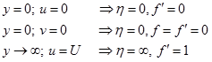(5.912)

The popular Runge-Kutta numerical technique can be applied for Eqs (5.9.11 & 5.9.12) to obtain the similarity solution in terms of and some of the values are given in the Table 5.9.1.