Characteristics Conditions
Consider an arbitrary flow field, in which a fluid element is travelling at some Mach number (M) and velocity (V) at a given point ‘A'. The static pressure, temperature and density are ![]() , respectively. Now, imagine that the fluid element is adiabatically slowed down
, respectively. Now, imagine that the fluid element is adiabatically slowed down ![]() or speeded up
or speeded up ![]() until the Mach number at ‘A' reaches the sonic state as shown in Fig. 4.3.2. Thus, the temperature will change in this process. This imaginary situation of the flow field when a real state in the flow is brought to sonic state is known as the characteristics conditions. The associated parameters are denoted as
until the Mach number at ‘A' reaches the sonic state as shown in Fig. 4.3.2. Thus, the temperature will change in this process. This imaginary situation of the flow field when a real state in the flow is brought to sonic state is known as the characteristics conditions. The associated parameters are denoted as ![]() etc.
etc.
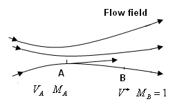
Fig. 4.3.2: Illustration of characteristics states of a gas.
Now, revisit Eq. (4.3.2) and use the relations for a calorically perfect gas, by replacing, ![]() . Another form of energy equation is obtained as below;
. Another form of energy equation is obtained as below;
(4.3.7) |
At the imagined condition (point 2) of Mach 1, the flow velocity is sonic and ![]() . Then the Eq. (4.3.7) becomes,
. Then the Eq. (4.3.7) becomes,
 |
(4.3.8) |
Like stagnation properties, these imagined conditions are associated properties of any fluid element which is actually moving with velocity u. If an actual flow field is non-adiabatic from ![]() , then
, then ![]() .On the other hand if the general flow field is adiabatic throughout, then
.On the other hand if the general flow field is adiabatic throughout, then ![]() is a constant value at every point in the flow. Dividing u2 both sides for Eq. (4.3.8) leads to,
is a constant value at every point in the flow. Dividing u2 both sides for Eq. (4.3.8) leads to,
 |
(4.3.9) |
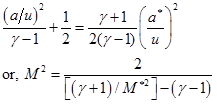
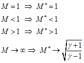
This equation provides the relation between actual Mach number (M) and characteristics Mach number ![]() . It may be shown that when M approaches infinity,
. It may be shown that when M approaches infinity, ![]() reaches a finite value. From Eq. (4.3.9), it may be seen that
reaches a finite value. From Eq. (4.3.9), it may be seen that
 |
(4.3.10) |