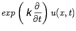
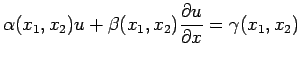
 |
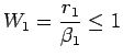
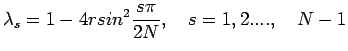
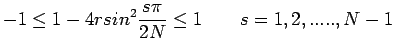
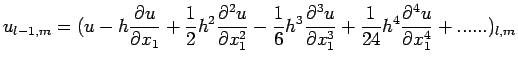
(1) |

 |
|||
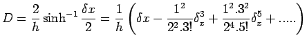
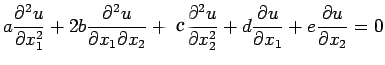
 |
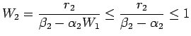
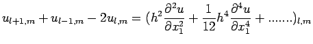
| (2) |
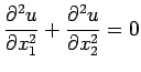
 |
(3) |
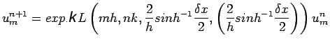 |
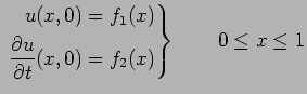
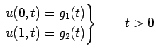
(4) |
 |
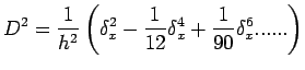
(5) |
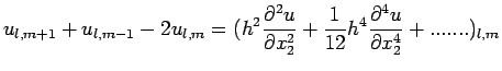
| (6) |
 |
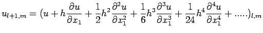
(7) |
![$\displaystyle u^{n+1}_{m}=\left[1+r\delta^{2}_{x} + \frac{1}{2}r\left(r-\frac{1}{6}\right)\delta^{4}_{x} + ...... \right]u^{n}_{m }$](img116.png) |
(8) |
 is the mesh ratio. From
equation (8), if we retain only second order central differences,
the forward difference formula
is the mesh ratio. From
equation (8), if we retain only second order central differences,
the forward difference formula
| (9) |
| (10) |
| (11) |

 |
(12) |
 |
(13) |
 |
(14) |
 |
(15) |
 |
(16) |

 |
(17) |
 |
(18) |
| (19) |
| (20) |
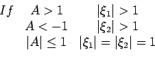
If |
(21) |
| (22) |
 |
| (23) |
 and
thus the method is stable if
and
thus the method is stable if

 |
(24) |
 |
 |
 |
(27) |
| (28) |
![$\displaystyle T^{n}_{m}=K^{2}h^{2}\left[\frac{1}{12}(p^{2}-1)\frac{\partial^{4}...
...^{2}(p^{4}-1)+
\frac{\partial^{6}u(x_{m},t_{n})}{\partial x^{6}}+.......\right]$](img260.png)
![$\displaystyle U^{1}_{m}=(1-p^{2})f_{1}(mh)+Kf_{2}(mh)+\frac{1}{2}p^{2}[f_{1}(m-1)h+f_{1}(m+1)h]\quad 1\leq
m\leq M-1$](img268.png)
| (29) |
 .
.
 , one can examine this scheme for
stability and find that the scheme is stable for all
, one can examine this scheme for
stability and find that the scheme is stable for all ![$\displaystyle =\frac{4}{p^{2}}\left[U^{n+1}_{m}-2U^{n}_{m}+U^{n-1}_{m}\right]$](img289.png)
 as
as
 |
(30) |
| (31) |
 |
(32) |
 |
(33) |
 |
(34) |
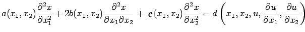
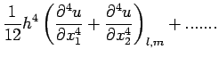
![$\displaystyle u_{l+1,m}+u_{l-1,m}+u_{l,m+1}+u_{l,m-1}-4u_{l,m}=
\left[ h^{2}\le...
..._{1}^{4}}+\frac{\partial^{ 4}u}{\partial x_{2}^{
4}}\right)+......\right]_{l,m}$](img319.png)
| (35) |
| (36) |