Differentiation Formulas:

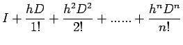
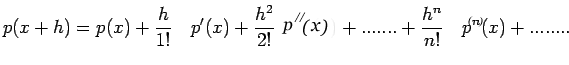
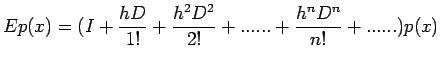
In order to obtain formulas for numerical differentiation, by operational methods, it is necessary to relate D (the differential operator) to the operators $\Delta,$ $\nabla$ and $\delta$ (delta operators). For this purpose, we notice that the familiar formula of the Taylor-series expansion

$$p(x+h)=p(x)+\frac{h}{1!}\quad p'(x)+\frac{h^{2}}{2!}\quad p''(x)+.......+\frac {h^{n}}{n!}\quad p^{n}(x)+........$$

(which certainly is valid for any polynomial) can be written in the operational form

$$E p(x)=(I+\frac{hD}{1!}+\frac{h^{2}D^{2}}{2!}+......+\frac{h^{n}D^{n}}{n!}+......)p(x)$$

$$=exp(hD)p(x)$$

and thus we deduce that

$$E=exp(hD)$$

which is to be interpreted as an abbreviation of the statement that the operators $E$ and $$I+\frac{hD}{1!}+\frac{h^{2}D^{2}}{2!}+......+\frac{h^{n}D^{n}}{n!}$$ are equivalent when applied to any polynomial $p_{{n}}(x)$ of degree $n$ for any n.
Further, we obtain the additional relations

$$hD = log E = log(I+\Delta)$$

$$=-log(I-\nabla)$$

$$= 2\quad log\left[\left(I+\frac{1}{4}\delta^{2}\right)^{\frac{1}{2}}+\frac{1}{2}\delta\right]$$

$$=2\quad sinh^{-1}\frac{\delta}{2}$$

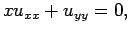
Classification of second order PDES':
The general linear second order partial differential equation in two independent variables is given by

$$A u_{xx}+2B u_{xy}+Cu_{yy}+Du_{x}+Eu_{y}+Fu+G=0$$

where the coefficients are functions of x and y and the subscripts denote partial derivatives with respect to the independent variables. The above equation is called

$$elliptic, \quad if \quad B^{2}-AC<0$$

$$parabolic, \quad if \quad B^{2}-AC=0$$

$$and \quad hyperbolic,\quad if \quad B^{2}-AC>0$$

This classification depends in general on the region of the $(x,y)$ plane under consideration. The differential equation
     $xu_{xx}+u_{yy}=0,$     for instance,    is elliptic for $x>0,$

$$hyperbolic for \quad x<0 \quad and$$

$$parabolic for \quad x=0 \quad$$

The well known examples of the three types are:
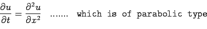
Heat Flow equation:

$$\begin{array}{ccc} \displaystyle \frac{\partial u}{\partial... ...&.......& \texttt{which is of parabolic type} \\ \end{array}%$$

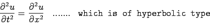
Wave equation:

$$\begin{array}{ccc} \displaystyle \frac{\partial^{2}u}{\part... ..........& \texttt{which is of hyperbolic type} \\ \end{array}%$$

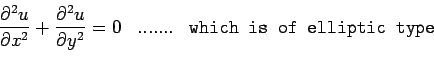
Laplace equation:

$$\begin{array}{ccc} \displaystyle \frac{\partial^{2}u}{\part... ...0&.......& \texttt{which is of elliptic type} \\ \end{array}%$$

The parabolic and hyperbolic type of equations are either initial value problems or initial boundary value problems whereas the elliptic type equation is always a boundary value problem. The boundary conditions can be one of the following three types:

1. The Disichlet or first boundary condition: Here, the solution is prescribed along the boundary
2. The Neumann or Second boundary condition: Here, the derivative of the solution is specified along the boundary.
3. The third a mixed boundary condition: Here, the solution and its derivative are prescribed along the boundary.