
Next:Hyperbolic Equation Up:Main
Previous:Solution of Tridiagonal systems:
Convergence:
The problem of convergence of a finite difference method for solving equation (1) consists of finding the condition under which
The difference between the exact solutions of the differential and difference equations at a fixed point  , tends to zero uniformly, as the net is refined in such a way that
  and
and
 , with
  and
and  remaining fixed. The fixed point is anywhere within the region
  under consideration, and it is sometimes convenient in the convergence analysis to assume that
  do not tend to zero independently but according to some relationship like
 |
(19) |
where  is a constant.
As an example of a convergence analysis for difference formula (10), we introduce
the difference between the theoretical (exact) solutions of the differential and difference equations at the grid point X=mh, T=nk. From equation (12), this satisfies the equation

If , the coefficients on the right hand side of equation (20) are all non-negative and so
where A depends on the upper bounds for
 and
and
 and
and  is the maximum modulus value of
  over the required range of
  . Thus
and so if  (the same initial data for differential and difference equations),
 as
as
 for fixed
  . This establishes convergence if the expression (21) is satisfied.
Stability:
The problem of stability of a finite difference scheme for solving equation (1) consists of finding conditions under which
the difference between the theoretical and numerical solutions of the difference equation, remains bounded as  increases, k remaining fixed for all . There are two methods which are commonly used for examining stability of a finite difference scheme.
Von Neumann Method:
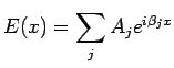
In this method, a harmonic decomposition is made of the error Z at grid points, at a given time level, leading to the error function.
where in general the frequencies
 and
and  are arbitrary. It is necessary to consider only the single term
 where
where  is any real number. For convenience, suppose that the time level being considered corresponds to t=0. To investigate the error propagation as t increases, it is necessary to find a solution of the finite difference equation which reduces to
when t=0. Let such a solution be
where
is any real number. For convenience, suppose that the time level being considered corresponds to t=0. To investigate the error propagation as t increases, it is necessary to find a solution of the finite difference equation which reduces to
when t=0. Let such a solution be
where
 is, in general, complex. The original error component
will not grow with time if
is, in general, complex. The original error component
will not grow with time if
 for all
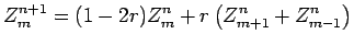
  . This is Von Neumann criterion for stability. As an example, let us examine the stability of finite difference scheme (10). Since satisfies the original difference equation, we get
 |
(22) |
Let
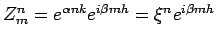 , where
 . Then equation (22) gives
Cancelling
. Then equation (22) gives
Cancelling
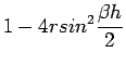
 on both sides leads to
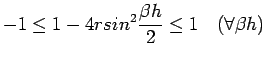
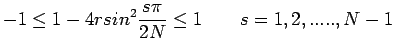
The quantity x is called the amplification factor. For stability,
 , for all values of
  , and so
The right hand side of the inequality is satisfied if
, and so
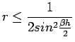
The right hand side of the inequality is satisfied if  and the left hand side gives
leading to the stability condition
and the left hand side gives
leading to the stability condition
 .
.
The Matrix Method:
If  , the totality of difference equations connecting values of U at two neighboring time levels can be written in the matrix form
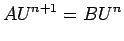 |
(23) |
where
 denotes the column vector
and A,B are square matrices of order
denotes the column vector
and A,B are square matrices of order  . If the difference formula is explicit A=I. Now equation (23) can be written in the explicit form
where
. If the difference formula is explicit A=I. Now equation (23) can be written in the explicit form
where  provided
  . The error vector
satisfies
from which it follow that
. The error vector
satisfies
from which it follow that
Where

denotes a suitable norm. The necessary and sufficient condition for the stability of a finite difference scheme based on a constant time step and proceeding indefinitely in time is

. When

is symmetric,
where
are the eigen values of
, and

denotes the

norm. As an example of the matrix method for examining stability , we consider the finite difference scheme (10). Here we have,
The eigen values of this matrix are
and thus the method is stable if
an identical condition obtained by the method of Von Neumann.
A difference approximation to a parabolic equation is consistent, if truncation error 
as
.
Next:Hyperbolic Equation Up:Main
Previous:Solution of Tridiagonal systems: