
Next: Newton-Gregory Backward Difference
Up: Main: Previous: Newton Divided Difference Table:
Newton Interpolation polynomial with equidistant points:
Gregory-Newton Forward Difference Approach:
Very often it so happens in practice that the given data set
 correspond to a sequence
  of
equally spaced points. Here we can assume that
of
equally spaced points. Here we can assume that
 |
(1) |
where

is the starting point (sometimes, for convenience,
the middle data point is taken as
and in such a case the
integer

is allowed to take both negative and positive values.)
and

is the step size. Further it is enough to calculate simple
differences rather than the divided differences as in the
non-uniformly placed data set case. These simple differences can
be forward differences

or backward differences

. We will first look at forward differences and
the interpolation polynomial based on
forward differences.
The first order forward difference

is defined as
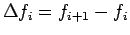 |
(7.1) |
The second order forward difference
 is defined
as
is defined
as
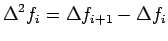 |
(7.2) |
The  order forward difference
 is
defined as
is
defined as
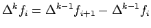 |
(7.3) |
Since we already know Newton interpolation polynomial in terms of
divided differences, to derive or generate Newton interpolation
polynomial in terms of forward differences it is enough to express
forward differences in terms of divided differences.
Recall the definition of first divided difference
![$ f[x_{0},x_{1}]$](img212.png)
,
![$\displaystyle f[x_{0},x_{1}]=\frac{f(x_{1})-f(x_{0})}{x_{1}-x_{0}}=\frac{f_{1}-f_{0}}{h}=\frac{\Delta
f_{0}}{h}$](img213.png)
![% latex2html id marker 2670
$\displaystyle \therefore \Delta f_{0}=hf[x_{0},x_{1}]$](img214.png) |
(8.1) |
Similarly we can get
![$\displaystyle \Delta f_{1}= hf[x_{1},x_{2}]$](img215.png) |
(8.2) |
By the definition of second order forward difference
 , we get
In a similar way, in general, we can show that
![$\displaystyle \Delta^{k}f_{i}=k!h^{k}f[x_{i},x_{i+1},x_{i+2}...x_{i+k}]$](img223.png) |
(8.4) |
![% latex2html id marker 2701
$\displaystyle \therefore f[x_{i},x_{i+1},...x_{i+k}]=\frac{\Delta^{k}f_{i}}{k!h^{k}}$](img224.png) |
(8.5) |
For  ,
,
![$\displaystyle f[x_{0},x_{1}...x_{k}]=\frac{\Delta^{k}f_{0}}{k!h^{k}}$](img226.png) |
(8.6) |
Now using (6.1) & (8.6) the Newton forward difference interpolation
polynomial may be written as follows:
 |
(9) |
To rewrite (9) in a simpler way let us set
i.e |
 |
(10) |
where
This is known as Newton-Gregory forward difference interpolation
polynomial. For convenience while constructing (10) one can first
generate a forward difference table and use the
from the table. Suppose we have data set

,
then forward difference table looks as follows:
Given the following data, estimate  using Newton-Gregory forward difference interpolation polynomial:
| i |
0 |
1 |
2 |
3 |
4 |
 |
1.0 |
3.0 |
5.0 |
7.0 |
9.0 |
 |
0 |
1.0986 |
1.6094 |
1.9459 |
2.1972 |
Solution:
Here we have five data points i.e
 Let us first generate the forward difference table.
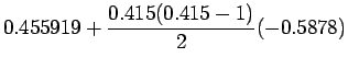
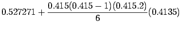
 Newton Gregory forward difference interpolation
polynomial is given by:
Newton Gregory forward difference interpolation
polynomial is given by:
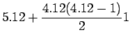
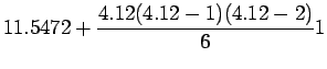
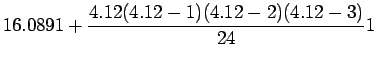
Example 2:
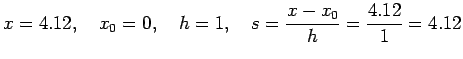
Given the following data estimate f(4.12)
using Newton-Gregory forward difference interpolation
polynomial:
| i |
0 |
1 |
2 |
3 |
4 |
5 |
|
0 |
1 |
2 |
3 |
4 |
5 |
|
1 |
2 |
4 |
8 |
16 |
32 |
Solution:
Let us first generate the Newton-Gregory forward
difference table:
Here
We know that the forward difference interpolation polynomial is
given by:
Exercise: Calculate  using Newton-Gregory forward difference formula for the following data
1)
x |
10 |
20 |
30 |
40 |
50 |
f(x) |
0.1736 |
0.3420 |
0.5000 |
0.6428 |
0.7660 |
and 
2)
x |
1.0 |
2.0 |
3.0 |
4.0 |
f(x) |
0.0 |
0.6931 |
1.0986 |
1.3863 |
and 
Next: 2.3.2 Newton-Gregory Backward Difference
Up: Main:Previous: 2.3 Newton Divided Difference Table:
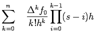
![$\displaystyle \sum\limits_{k=0}^{n}\quad\frac{\Delta^{k}f_{0}}{k!h^{k}}\quad[s(s-1).......(s-k+1)]h^{k}$](img233.png)