(2.2.2)Newton Divided Difference Table:

It may also be noted for calculating the higher order divided differences we have used lower order divided differences. In fact starting from the given zeroth order differences ; one can systematically arrive at any of higher order divided differences. For clarity the entire calculation may be depicted in the form of a table called

Newton Divided Difference Table.

Again suppose that we are given the data set $(x_{i},f_{i}),$ and that we are interested in finding the $5^{th}$ order Newton Divided Difference interpolynomial. Let us first construct the Newton Divided Difference Table. Wherein one can clearly see how the lower order differences are used in calculating the higher order Divided Differences:

Solution:
Here

. One can fit a fourth order Newton Divided Difference interpolation polynomial to the given data. Let us generate Newton Divided Difference Table; as requested.

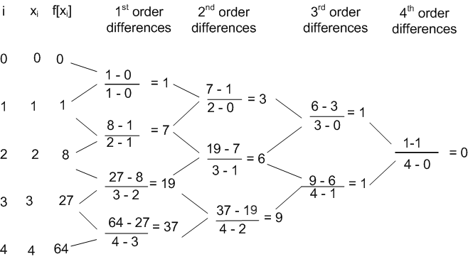
Note: One may note that the given data corresponds to the cubic polynomial

. To fit such a data $3^{rd}$ order polynomial is adequate. From the Newton Divided Difference table we notice that the fourth order difference is zero. Further the divided differences in the table can be directly used for constructing the Newton Divided Difference interpolation polynomial that would fit the data.

Exercise: Using Newton divided difference interpolation polynomial , construct polynomials of degree two and three for the following data:

(1) f(8.1) = 16.94410, f(8.3)=17.56492 , f(8.6) = 18.50515, f(8.7) = 18.82091.

(2) f(0.6) = -0.17694460 , f(0.7) = 0.01375227 , f(0.8) = 0.22363362 , f(1.0) = 0.65809197.

i	1	2	3	4
$x_{i}$	1	2	3	4
$y_{i}=f(x_{i})$	1	8	27	64