
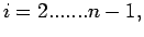
Next: Newton Interpolation polynomial:
Up: Main:Previous: Introduction:
Interpolation
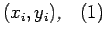
Let us suppose that the given
data points


is coming from a
function

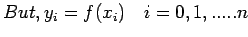
. Let us assume that this function

takes
the values
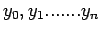
at
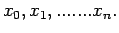
Since there are

data points
we can represent the function
by a
polynomial of degree

 |
(1) |
As we have assumed that
 i.e. the
function passes through
i.e. the
function passes through
 can be
rewritten as:
can be
rewritten as:
 |
(2) |
 |
(3) |
Using (3) for i=0, in (2) we get
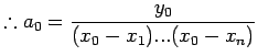 |
(4.1) |
For  we get
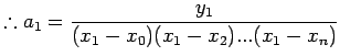 |
(4.2) |
Similarly for
 we get
and for
we get
and for  we get
 |
(4.3) |
Using (4.1)-(4.3) in (2) we get
 |
(5) |
 |
(6) |
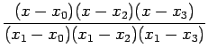
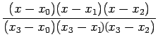
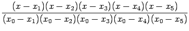
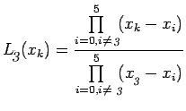
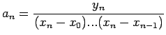
(5) can be rewritten in a compact form as:
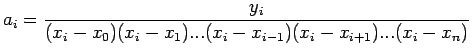
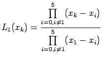
where
 |
(7.2) |
It can be easily noted that
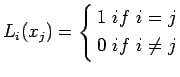 |
7.3 |
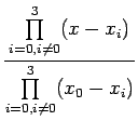
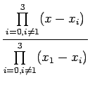
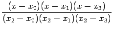
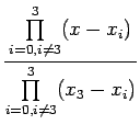
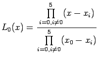
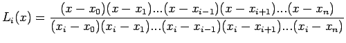
Let us introduce the product notation as :
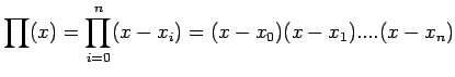 |
(8.1) |
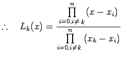 |
(8.2) |
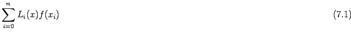
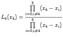
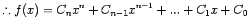
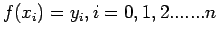
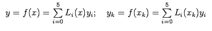
Therefore, Lagrange interpolation polynomial of degree n can be
written as
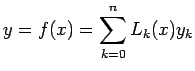 |
(9) |
Example 1:
Given the following data table, construct the
Lagrange interpolation
polynomial , to fit the data and find 
| i |
0 |
1 |
2 |
3 |
 |
0 |
1 |
2 |
3 |
 |
1 |
2.25 |
3.75 |
4.25 |
Solution:
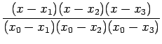
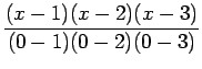
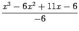
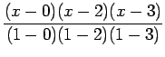
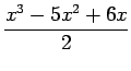
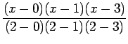
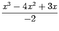
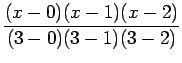
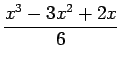
Here  .
.
 Lagrange interpolation polynomial is given by
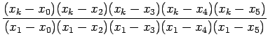
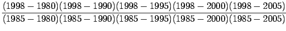
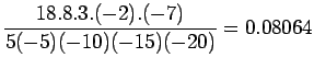
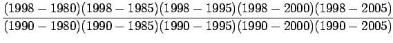
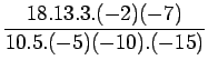
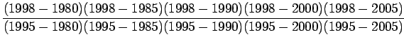
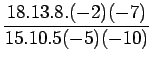
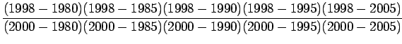
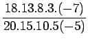
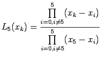
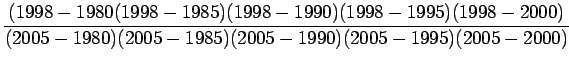
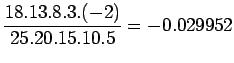
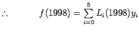
Example 2:
Given the following data table, construct the
Lagrange interpolation polynomial f(x), to fit the data and find 
| i |
0 |
1 |
2 |
3 |
4 |
5 |
|
1980 |
1985 |
1990 |
1995 |
2000 |
2005 |
|
|
440 |
510 |
525 |
571 |
500 |
600 |
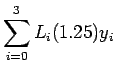
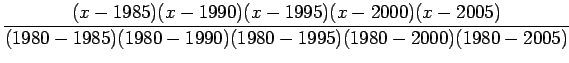
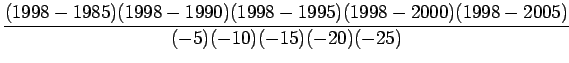
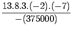
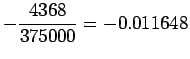
Solution:
Here
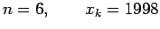
Lagrange interpolation polynomial is given by
Next: Newton Interpolation polynomial:Up: Main:
Previous: Introduction: