
Next: Least Squares Regression (Continued) Up :Main Previous :Newton-Gregory Backward Difference Interpolation polynomial:
Least-Squares Regression
Let us suppose that the given data
![]() ,
, ![]() is
inexact and has substantial error, right from their source where
they are obtained. Experimental data is usually scattered and is a
good example for inexact data. Polynomial interpolation is
inappropriate in such cases. To understand this let us look at the
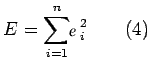
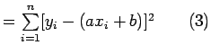
following graphical representation of some scattered data:
is
inexact and has substantial error, right from their source where
they are obtained. Experimental data is usually scattered and is a
good example for inexact data. Polynomial interpolation is
inappropriate in such cases. To understand this let us look at the
following graphical representation of some scattered data:
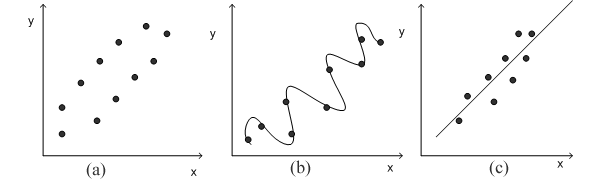
Fig :1(a) Scattered Data;
Fig :1(b) A polynomial fit oscillating beyond the range of the data;
Fig :1(c) An approximate fit for data.
Now a look at the data in figure 1(a) tells us that the data has increasing trend i.e. higher values of y are associated with higher values of x. As in figure 1(b) if we fit an eigth order interpolation polynomial, it passes through the data exactly but oscillates due to the scattered nature of data and also goes well beyond the range suggested by data. Hence a more appropriate way is to find a function as shown in fig 1(c), that fits the shape or general trend of the data. One of the standard techniques for finding such a fit is Least-Square Regression.
2.4.1 Least Square Method:
The principle of least squares is one of the popular methods for
finding a curve fitting a given data. Say
![]() ,
,
![]() be n observations from an
experiment. We are interested in finding a curve
be n observations from an
experiment. We are interested in finding a curve
![]()
Closely fitting the given data of size 'n'. Now at ![]() while
the observed value of
while
the observed value of ![]() is
is ![]() , the expected value of
, the expected value of ![]() from the
curve
from the
curve ![]() is
is ![]() . Let us define the residual by
. Let us define the residual by
Likewise, the residuals at all other points
![]() are
given by
are
given by
![]()
....................(3)
...........................
Some of the residuals ![]() may be positive and some may be
negative. We would like to find the curve fitting the given data
such that the residual at any
may be positive and some may be
negative. We would like to find the curve fitting the given data
such that the residual at any ![]() is as small as possible. Now
since some of the residuals are positive and others are negative
and as we would like to give equal importance to all the residuals
it is desirable to consider sum of the squares of these residuals,
say
is as small as possible. Now
since some of the residuals are positive and others are negative
and as we would like to give equal importance to all the residuals
it is desirable to consider sum of the squares of these residuals,
say ![]() and thereby find the curve that minimizes
and thereby find the curve that minimizes ![]() . Thus, we
consider
. Thus, we
consider
and find the best representative curve (1) that minimizes (4).
2.4.2 Least Square Fit of a Straight Line
Suppose that we are given a data set
![]() of
of ![]() observations from an experiment. Say that we are interested
in fitting a straight line
observations from an experiment. Say that we are interested
in fitting a straight line
![]()
to the given data. Find the '![]() ' residuals
' residuals ![]() by:
by:
![]()
Now consider the sum of the squares of ![]() i.e
i.e

Note that ![]() is a function of parameters a and b. We need to find a,b such that
is a function of parameters a and b. We need to find a,b such that ![]() is minimum. The necessary condition for
is minimum. The necessary condition for ![]() to be minimum is given by:
to be minimum is given by:
![]()
The condition ![]() yields:
yields:
i.e 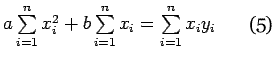
Similarly the condition ![]() yields
yields
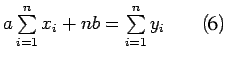
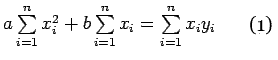
Equations (5) and (6) are called as normal equations,which are to be solved to get desired values for a and b.
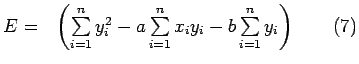
The expression for ![]() i.e (3) can be re-written in a convenient way as follows:
i.e (3) can be re-written in a convenient way as follows:
Example: Using the method of least squares, find an equation of the form
![]() that fits the following data:
that fits the following data:
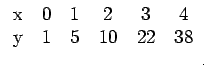
Solution: Consider the normal equations of least square fit of a straight line i.e
Here ![]() =5.
=5.
From the given data, we have,
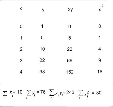
Therefore the normal equations are given by:
30a +10b =243 ................(3)
10a+5b=76.......................(4)
On solving (3) and (4) we get
a = 9.1 , b= - 3 ................................................................(5)
Hence the required fit for the given data is
y=9.1x - 3 ...................... ..(6)
![]()
![]()
Next: Least Squares Regression (Continued) Up :Main
Previous :Newton-Gregory Backward Difference Interpolation polynomial: