Next: Nonlinear Regression Up: Main Previous:Least Squares Regression

Least -Squares Regression ...(continued)

Remarks:

(1) Experimental data may not be always linear. One may be interested in fitting either a curve of the form $(a)$ $y=ax^{b}$ or $(b)$ $y = ae^{bx}$ However, both of these forms can be linearized by taking logarithms on both the sides. Let us look at the details:

On taking logarithms on both the sides we get:

Say                             

Using (3) in (2) we get

which is linear in .

On taking logarithms we get

Say                           

we get

which is linear in $Y, x$

Example: By the method of least square fit a curve of the form $y=ax^{b}$ to the following data:

Solution.

Consider $y=ax^{b}\qquad(1)$

On taking logarithm on both the sides we get

Say                                   

Using (3) in (2) we get

Data in modified variables

Normal equations corresponding to the straight line fit (4) are:

From the modified data we get

normal equations take the form:

On solving for we obtain,

$b=1.9311, \quad A=0.8678.$

.

The desired curve is

Least Square fit of a parabola

Given a data set of n observations $(x_{i},y_{i})$, of an experiment .Now we try to fit a best possible parabola

$y=ax^{2}+bx+c\qquad(1)$

following the principle of least square. Finding the appropriate parabola amounts to determining the constants $a, b, c$ that minimize the sum of the squares of the residuals given by

The necessary condition for E to be minimum is

$$\frac{\partial E}{\partial a}=\frac{\partial E}{\partial b}=\frac{\partial E}{\partial c}=0\qquad(3)$$

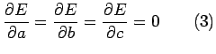
Now the condition yields

$$\frac{\partial E}{\partial a}=-\sum\limits_{i=1}^{n}2[y_{i}-(ax^{2}_{i}+bx_{i}+c)](x^{2}_{i})=0$$

i.e                               $$a\sum\limits_{i=1}^{n}x^{4}_{i}+b\sum\limits_{i=1}^{n}x^{3}_{i}+c\sum\limits_{i=1}^{n}x^{2}_{i}=\sum\limits_{i=1}^{n}x_{i}^{2}y_{i}\qquad(4)$$

Similarly yields

$$\frac{\partial E}{\partial b}=-\sum\limits_{i=1}^{n}2[y_{i}-(ax^{2}_{i}+bx_{i}+c)]x_{i}=0$$

i.e                                     $$a\sum\limits_{i=1}^{n}x^{3}_{i}+b\sum\limits_{i=1}^{n}x^{2}_{i}+c\sum\limits_{i=1}^{n}x_{i}=\sum\limits_{i=1}^{n}x_{i}y_{i}\qquad(5)$$

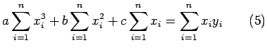
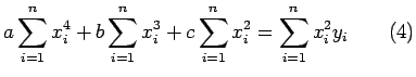
Finally yields

$a\sum\limits_{i=1}^{n}x^{2}_{i}+b\sum\limits_{i=1}^{n}x_{i}+nc=\sum\limits_{i=1}^{n}y_{i}\qquad(6)$

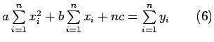
Equations (4), (5) and (6) are called as normal equations whose solution yields the values of the constants a, b and c and thus the desired parabola.

Example: Given the following data from an experimental observation

y:	9.4	11.8	14.7	18.0	23.0
x:	1.0	1.6	2.5	4.0	6.0

fit a parabola in the form $y=ax^{2}+bx+c$ following the principle of least square.

Solution) Here

The normal equations for finding a parabolic fit are:

$a\sum\limits_{i}x^{4}_{i}+b\sum\limits_{i}x_{i}^{3}+c\sum\limits_{i}x^{2}_{i}=\sum\limits_{i}x^{2}_{i}y_{i}$	(1)
$a\sum\limits_{i}x^{3}_{i}+b\sum\limits_{i}x_{i}^{2}+c\sum\limits_{i}x_{i}=\sum\limits_{i}x_{i}y_{i}$

The normal equations are:

$1598.6161 a+110.721 b+61.81 c=1247.483$
$110.721 a + 61.81 b +15.1 c = 275.03$	(2)

On Solving (2) for $a, b, c,$ we get

Next: Nonlinear Regression Up: Main Previous:Least Squares Regression