
Next:Approx. and Round-off-Errors Up :Main Previous : Least Squares Regression (continued)
Nonlinear Regression:
Next:Approx. and Round-off-Errors Up :Main Previous : Least Squares Regression (continued)
Nonlinear Regression:
Suppose that we are interested in fitting a curve of the form
to a given data set of ![]() observations from an experiment. Unlike
the transcendental curve or exponential curve one cannot linearize
observations from an experiment. Unlike
the transcendental curve or exponential curve one cannot linearize
![]() by taking logarithms on both the sides. However, like in
linear regression analysis, nonlinear regression is based on
determining the values of the parameters that minimize the sum of
the squares of residuals. In the nonlinear case this is achieved
in a iterative fashion.
by taking logarithms on both the sides. However, like in
linear regression analysis, nonlinear regression is based on
determining the values of the parameters that minimize the sum of
the squares of residuals. In the nonlinear case this is achieved
in a iterative fashion.
The Gauss-Newton method is used for minimizing the sum of the squares of the residuals between data and nonlinear equations. Here the Taylor series expansion is used to express the original nonlinear equation in an approximate, linear form. Then the principle of least square is used to obtain new estimates of the parameters that move in the direction of minimizing the residual.
Now to illustrate the methodology let us represent ![]() as
as
Let us suppose that we are given a data set
![]() ...
...
![]() of
of ![]() observations from an experiment. At each of
observations from an experiment. At each of
![]() while
while
![]() is the measured value ,
is the measured value ,
![]() will be the
estimated value. For simplicity we denote
will be the
estimated value. For simplicity we denote
![]() by
by ![]() . Now going by the Gauss-Newton method , let us
linearize the nonlinear mode at
. Now going by the Gauss-Newton method , let us
linearize the nonlinear mode at
![]() iteration level using
Taylor series as follows:
iteration level using
Taylor series as follows:
![]()
where the subscripts ![]() denote iteration levels,
denote iteration levels,
![]()
Now we may note that ![]() represents the linearized version of
the model w.r.t iteration level.
represents the linearized version of
the model w.r.t iteration level. ![]() at
at
![]() iteration
we already know the
iteration
we already know the ![]() level values of the parameters i.e
level values of the parameters i.e ![]() &
& ![]() . Now we have the residuals
. Now we have the residuals ![]() given by :
given by :
![]()
![]()
which in the matrix form may be written as
![]()
where
![]()
![]() is the matrix of partial derivatives of the
function evaluated with the
is the matrix of partial derivatives of the
function evaluated with the ![]() level iteration values.
level iteration values.
 ,
,
![]()
![]() contains the differences between the measurements and
the function values and
contains the differences between the measurements and
the function values and
![]() contains the changes in the
parameter values.
contains the changes in the
parameter values.
Applying the principle of least squares on ![]() we arrive at
we arrive at
![]()
Now on solving ![]() we obtain
we obtain
![]() , which can be used
to compute improved values of the parameters
, which can be used
to compute improved values of the parameters
![]()
![]()
![]()
We repeat the above procedure until the solution converges i.e until
![]() (10)
(10)
where
![]() denotes the relative error in
denotes the relative error in
![]() parameter and
parameter and
![]() is
some prescribed tolerance level for the relative error in
is
some prescribed tolerance level for the relative error in
![]() parameter.
parameter.
Example: Fit the function
![]() to the
following data:
to the
following data:
Using the initial guesses of
![]() , find the
solution to an accuracy of
, find the
solution to an accuracy of ![]()
Solution) The partial derivatives of the function w.r.t
![]() are:
are:
![]()
Given that
![]()
using
![]()
![]() and the given data we get
and the given data we get
![\begin{displaymath}
% latex2html id marker 694
\therefore[Z^{T}_{0}][Z_{0}]=\lef...
....3193 & 0.9489 \\
0.9489 & 0.4404 \\
\end{array}%
\right]\end{displaymath}](img53.png)
![\begin{displaymath}
% latex2html id marker 696
\therefore\left[[Z_{0}^{T}][Z_{0}...
...97 & - 7.8421\\
-7.8421 & 19.1678 \\
\end{array}%
\right]\end{displaymath}](img54.png)
Using ![]() and given data we get
and given data we get
 =
=
![\begin{displaymath}
% latex2html id marker 704
\therefore \{Z_{0}^{T}\}\{D\}=\le...
...in{array}{c}
-0.1533 \\
-0.0365 \\
\end{array}%
\right]\end{displaymath}](img58.png)
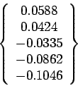
![]() By
By ![]() we get
we get
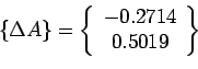
 =
=
 +
+

 +
+
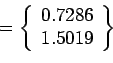
Now we start with
 and repeat the procedure to obtain

and so on till the convergence criteria ![]() is satisfied with
is satisfied with
![]() .
.
Remark:
(1) The partial derivatives
![]() may be calculated using difference equations i.e.
may be calculated using difference equations i.e.
Where ![]() small perturbation in
small perturbation in ![]() .
.
![]() are m+1 parameters.
are m+1 parameters.
![]() The Gauss-Newton method may converge slowly or may sometimes
oscillate widely or may not even converge. Modifications of the
method have been suggested to overcome the shortcomings. This
discussion is out of scope of the current discussion.
The Gauss-Newton method may converge slowly or may sometimes
oscillate widely or may not even converge. Modifications of the
method have been suggested to overcome the shortcomings. This
discussion is out of scope of the current discussion.
![]()
![]()
Next:Approx. and Round-off-Errors Up :Main Previous : Least Squares Regression (continued)