Next: Miscellaneous Remarks Up: Differential Equations Previous: Integrating Factors Contents
Some times we might think of a
subset or subclass of differential equations which admit explicit
solutions. This question is pertinent when we say that there are
no means to find the explicit solution of
 where
where ![]() is an arbitrary
continuous function in
is an arbitrary
continuous function in ![]() in suitable domain of definition.
In this context, we have a class of equations, called Linear
Equations (to be defined shortly) which admit explicit solutions.
in suitable domain of definition.
In this context, we have a class of equations, called Linear
Equations (to be defined shortly) which admit explicit solutions.
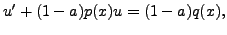
A first order equation is called a non-linear equation (in the independent variable) if it is neither a linear homogeneous nor a non-homogeneous linear equation.
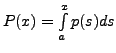
Define the indefinite integral
![]() ( or
( or
 ). Multiplying
(7.4.1) by
). Multiplying
(7.4.1) by  we get

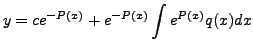
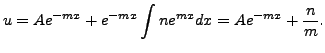
On integration, we get
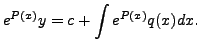
In other words,
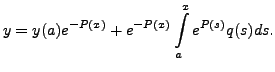
As a simple consequence, we have the following proposition.
 (where
Hence,
We can just use the second part of the above proposition to get the above
result, as ![]()
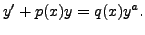
A class of nonlinear Equations (7.4.1) (named after
Bernoulli
![]() ) can be reduced to linear equation.
These equations are of the type
) can be reduced to linear equation.
These equations are of the type
 then (7.4.5) is a linear equation. Suppose
that
then (7.4.5) is a linear equation. Suppose
that
or equivalently
 constants and

and its solution is
Equivalently
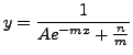
with

A K Lal 2007-09-12