Next: Diagonalisation Up: Eigenvalues, Eigenvectors and Diagonalisation Previous: Eigenvalues, Eigenvectors and Diagonalisation Contents
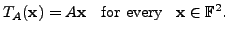
In this chapter, the linear transformations are from a
given finite dimensional vector space ![]() to itself. Observe
that in this case, the matrix of the linear transformation is a square
matrix. So, in this chapter, all the matrices
are square matrices and a vector
to itself. Observe
that in this case, the matrix of the linear transformation is a square
matrix. So, in this chapter, all the matrices
are square matrices and a vector
![]() means
means
 for some positive integer
 ![]()
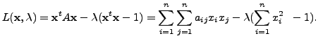
To solve this, consider the Lagrangian
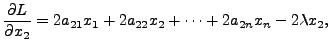
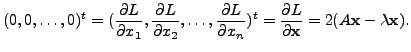
Partially differentiating

and so on, till
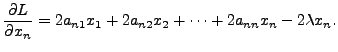
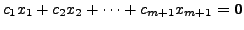
Therefore, to get the points of extrema, we solve for
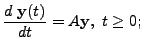
We therefore need to find a
Let ![]() be a matrix of order
be a matrix of order ![]() In general, we ask the question:
In general, we ask the question:
For what values of
![]() there exist a non-zero
vector
there exist a non-zero
vector
![]() such that
such that
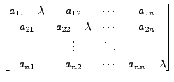
By Theorem 2.5.1, this system of linear equations has a non-zero solution, if
So, to solve (6.1.4), we are forced to choose those values of
Some books use the term EIGENVALUE in place of characteristic value.
has a non-zero solution. height6pt width 6pt depth 0pt
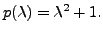
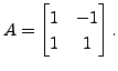
Consider the matrix
 Then the characteristic polynomial of
 ![]() is
is
Given the matrix
 and
and
 as eigenpairs.
 are
eigenvectors of
are
eigenvectors of  ,
then
,
then
 is
also an eigenvector of
is
also an eigenvector of
Suppose
![]() is a root of the characteristic equation
is a root of the characteristic equation
![]() Then
Then
![]() is singular and
is singular and
![]() Suppose
Suppose
![]() Then by Corollary 4.3.9,
the linear system
Then by Corollary 4.3.9,
the linear system
![]() has
has ![]() linearly
independent solutions. That is,
linearly
independent solutions. That is, ![]() has
has ![]() linearly independent
eigenvectors corresponding to the eigenvalue
linearly independent
eigenvectors corresponding to the eigenvalue
![]() whenever
whenever
![]()
 Then
Then
 That is
  is
equivalent to the equation
is
equivalent to the equation  And this has the solution
 Hence, from the above remark,
 Then
Then
 from
from
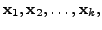
In general, if
![]() are linearly independent vectors
in
are linearly independent vectors
in
![]() then
then
![]() are
eigenpairs for the identity matrix,
are
eigenpairs for the identity matrix, ![]()
 Then
Then
 Now check that the
eigenpairs are
Now check that the
eigenpairs are
 In this
case, we have TWO DISTINCT EIGENVALUES AND THE CORRESPONDING
EIGENVECTORS ARE ALSO LINEARLY INDEPENDENT. The reader is required to prove
the linear independence of the two eigenvectors.
In this
case, we have TWO DISTINCT EIGENVALUES AND THE CORRESPONDING
EIGENVECTORS ARE ALSO LINEARLY INDEPENDENT. The reader is required to prove
the linear independence of the two eigenvectors.
 Then
Then
 and
and

 and
and
[Hint: Recall that if the matrices ![]() and
and ![]() are similar, then there
exists a non-singular matrix
are similar, then there
exists a non-singular matrix ![]() such that
such that
![]() ]
]
 Then prove that
  (
(
 and
and
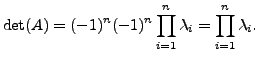
Also,
 the coefficient of
So,
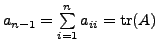 by definition of
trace.
by definition of
trace.
But , from (6.1.5) and (6.1.7), we get
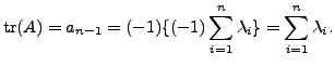
Hence, we get the required result. height6pt width 6pt depth 0pt
 Then prove that
0
is an eigenvalue of
Then prove that
0
is an eigenvalue of  .If
.If
Let ![]() be an
be an
![]() matrix.
Then in the proof of the above theorem, we observed that
the characteristic equation
matrix.
Then in the proof of the above theorem, we observed that
the characteristic equation
![]() is
a polynomial equation of degree
is
a polynomial equation of degree ![]() in
in
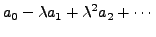
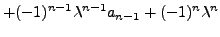
![]() Also, for some numbers
Also, for some numbers
![]() it has the form
it has the form
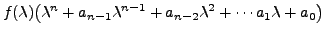
Note that, in the expression
It turns out that the expression
holds true as a matrix identity. This is a celebrated theorem called the Cayley Hamilton Theorem. We state this theorem without proof and give some implications.
holds true as a matrix identity.
Some of the implications of Cayley Hamilton Theorem are as follows.
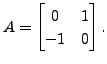
![$ A = \left[\begin{array}{cc}0&1 \\ 0 & 0
\end{array}\right].$](img2840.png) Then its characteristic polynomial is
Then its characteristic polynomial is
 where
where  and a polynomial
 |
|||
 |
That is, we just need to compute the powers of

In the language of graph theory, it says the following:
``Let ![]() be a graph on
be a graph on ![]() vertices. Suppose there is no path of length
vertices. Suppose there is no path of length
![]() or less from a vertex
or less from a vertex ![]() to a vertex
to a vertex ![]() of
of ![]() Then there is no
path from
Then there is no
path from ![]() to
to ![]() of any length. That is, the graph
of any length. That is, the graph ![]() is disconnected
and
is disconnected
and ![]() and
and ![]() are in different components."
are in different components."
![$\displaystyle A^{-1} = \frac{-1}{a_n} [ A^{n-1} + a_{n-1} A^{n-2} + \cdots + a_1 I ].$](img2861.png)
This matrix identity can be used to calculate the inverse.
 then the
set
then the
set
Let the result be true for
![]() We prove the result
for
We prove the result
for  We consider the equation
 We have
From Equations (6.1.9) and (6.1.10), we get
This is an equation in
But the eigenvalues are distinct implies
Thus, we have the required result. height6pt width 6pt depth 0pt
We are thus lead to the following important corollary.
 have the same set of eigenvalues.
 is
an eigenvalue of
is
an eigenvalue of  for any positive integer
 In each case, what can you say about the eigenvectors?
![$ [{\mathbf b}]_{{\cal B}} = (c_1, c_2, \ldots, c_n)^t$](img2901.png) then show that
then show that
A K Lal 2007-09-12