Euler's Method

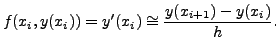
For a small step size $h$ , the derivative $y^\prime(h)$ is close enough to the ratio $$\frac{y(x+h) - y(x)}{h}$$ . In the Euler's method, such an approximation is attempted. To recall, we consider the problem (). Let $h = \displaystyle \frac{b-a}{n}$ be the step size and let $x_i = a + i h, 0 \le i \le n$ with $x_n = b$ . Let $y_k$ be the approximate value of $y$ at $x_k, \; k = 1, 2\ldots, n$ . We define

$$y_{k+1} = y_k + h f(x_k, y_k), \; k = 0, 1, 2, \ldots, n-1.$$ (14.1.2)

The method of determination of $y_k$ by () is called the EULER'S METHOD. For convenience, the value $f(x_k, y_k)$ is denoted by $f_k$ , for $k=0,1, 2, \ldots, n$ .

Remark 14.1.1  

1. Euler's method is an one-step method.
2. The Euler's method has a few motivations.
   1. The derivative $y^\prime$ at $x=x_i$ can be approximated by $$\frac{y(x_{i+1}) - y(x_i)}{h}$$ if $h$ is sufficiently small. Using such an approximation in (), we have
      $$f(x_i, y(x_i)) = y^\prime(x_i) \cong \frac{y(x_{i+1}) - y(x_i)}{h}.$$

   2. We can also look at () from the following point of view. The integration of () yields
      $$y(x_{i+1}) = y(x_i) + \int\limits_{x_i}^{x_{i+1}} f(x, y(x)) \; dx.$$
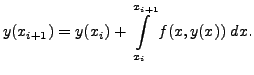
      The integral on the right hand side is approximated, for sufficiently small value of $h >0$ , by
      $$\int\limits_{x_i}^{x_{i+1}} f(s, y(x)) \; dx \cong f(x_i, y(x_i)) h.$$

   3. Moreover, if $y$ is differentiable sufficient number of times, we can also arrive at () by considering the Taylor's expansion
      $$y(x_{i+1}) = y(x_i) + h f(x_i, y(x_i)) + \frac{h^2}{2!} f(x_i, y(x_i)) + \cdots$$
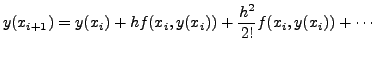
      and neglecting terms that contain powers of $h$ that are greater than or equal to $2$ .

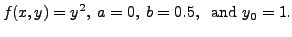
We illustrate the Euler's method with an example. The example is only for illustration. In (), we do not need numerical computation at each step as we know the exact value of the solution. The purpose of the example is to have a feeling for the behaviour of the error and its estimate. It will be more transparent to look at the percentage of error. It may throw more light on the propagation of error.

EXAMPLE 14.1.2   Use Euler's algorithm to find an approximate value of $y(1)$ , where $y$ is the solution of the IVP

$$y^\prime = y^2, \;\; y(0) = 1, \; 0 \le x \le 0.5$$ (14.1.3)

with step sizes $(i) \; 0.1$ and $(ii) \; 0.05.$ Show that the exact solution of the IVP is $y(x) = \displaystyle \frac{1}{1-x}$ . Calculate the error at each step and tabulate the results.
Solution: Comparing the given IVP with (), we note that

$$f(x,y) = y^2, \; a = 0, \; b=0.5, \; {\mbox{ and }} y_0 = 1.$$

The Euler's algorithm now reads as

$$y_{k+1} = y_k + h y_k^2, \; k=0,1,2,\ldots {\mbox{ and }} y_0 = 1.$$ (14.1.4)

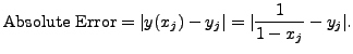
It is left as an exercise to verify that $y(x) = \displaystyle \frac{1}{1-x}$ is a solution of the given IVP. So, the absolute value of the error at the $j^{\mbox{th}}$ step is

$${\mbox{Absolute Error}} = \vert y(x_j) - y_j\vert = \vert \displaystyle \frac{1}{1 - x_j} - y_j\vert.$$

See the Tables  and for the calculation of errors (up to $5$ places of decimal).

		Table $1$
Initial $x$	Initial $y$	Step size $h$	Approx $y$	Exact $y$	Error
$0.00000$	1.00000	0.10000
$0.10000$	1.00000	0.10000	1.10000	1.11111	$0.01111$
0.20000	1.10000	0.10000	1.22100	1.25000	0.02900
0.30000	1.22100	0.10000	1.37008	1.42857	0.05849
0.40000	1.37008	0.10000	1.55780	1.66667	0.10887
0.50000	1.55780	0.10000	1.80047	2.00000	0.19953

		Table $2$
Initial $x$	Initial $y$	Step size $h$	Approx $y$	Exact $y$	Error
$0.00000$	1.00000	0.05000
$0.05000$	1.00000	0.05000	1.05000	1.05263	$0.00263$
0.10000	1.05000	0.05000	1.10513	1.11111	0.00599
0.15000	1.10513	0.05000	1.16619	1.17647	0.01028
0.20000	1.16619	0.05000	1.23419	1.25000	0.01581
0.25000	1.23419	0.05000	1.31035	1.33333	0.02298
0.30000	1.31035	0.05000	1.39620	1.42857	0.03237
0.35000	1.39620	0.05000	1.49367	1.53846	0.04479
0.40000	1.49367	0.05000	1.60522	1.66667	0.06144
0.45000	1.60522	0.05000	1.73406	1.81818	0.08412
0.50000	1.73406	0.05000	1.88441	2.00000	0.11559

Remark 14.1.3   At step $1$ , the approximation of the derivative induces a certain error. At the next step, the approximation of the derivative and the approximate value from the previous step can increase the error. This is what we see from the last column of the table. As mentioned earlier, the percentage of the error perhaps gives a better view of the accumulation of the error. With this in mind, we are tempted to have a look at the error estimates which is the topic of the ensuing section.

We now give a sample flow chart for the Euler's method.

Figure: Flow Chart for Euler's method