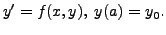
Next: Runge-Kutta Method Up: Numerical Methods Previous: Euler's Method Contents
When we develop a method, specially to get approximate values of a certain quantity, it is desirable to know how much of deviation we have made from the actual to the approximated value. This difference between the exact and the computed value is usually known as the error committed. An estimate for error also indicates how good is the calculated approximate value. In general, such a feature may not be possible. Euler's method is one such method which allows us for an analysis of the error, which is the main aim of this section. Note that we are not dealing with the truncation error in actual calculation. Recall that
 's are called the absolute error estimates,
committed at the
's are called the absolute error estimates,
committed at the
![[*]](crossref.png) ) be a twice continuously differentiable
function on )
at
) be a twice continuously differentiable
function on )
at 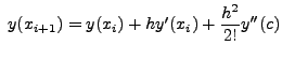 for some
  . Also, by Euler's method,
)) reduces to
. Also, by Euler's method,
)) reduces to
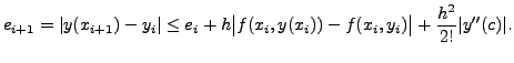
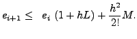
 is the solution of the difference equation
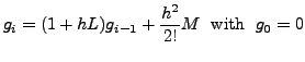 then
then
 for
for
 .
.
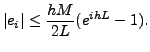
) implies that the error is in the class also gives
an upper bound for the estimate of the error at does not throw any light on the estimate of
global error.A K Lal 2007-09-12