Next: Euler's Method Up: Numerical Methods Previous: Numerical Methods Contents
This chapter attempts to describe a few methods for finding approximate values of a solution of a non-linear initial value problems. By no means, it is not an exhaustive study but can be looked upon as an introduction to numerical methods. Again, we stress that no attempt is made towards a deeper analysis. A question may arise: why one needs numerical methods for differential equations. Probably because, differential equations play an important role in many problems of engineering and science. This is so because the differential equations arise in mathematical modelling of many physical problems. The use of the numerical methods have become vital in the absence of explicit solutions. Normally, numerical methods have two major roles:
In this chapter, we do not enter into the aspect of error analysis. For the present, we deal with some of the numerical methods to find approximate value of the solution of initial value problems (IVP's) on finite intervals. We also mention that no effort is made to study the boundary value problems. Let us consider an initial value problem
![[*]](crossref.png) ) has a unique solution.
Our aim is to determine
) has a unique solution.
Our aim is to determine
we know the value of
), we
determine the approximate value of
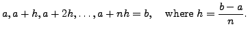
The number ![]() is called the step size and
is called the step size and ![]() depends on
depends on ![]() and
and ![]() .
For
.
For
![]() ,
the value of
,
the value of ![]() at
at ![]() is
is
![]() and its approximate value is denoted by
and its approximate value is denoted by ![]() .
In this chapter, we develop methods for determining an approximate value of
.
In this chapter, we develop methods for determining an approximate value of ![]() which is denoted
by
which is denoted
by  . This is achieved by evaluating the approximate values
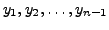 .
Normally
.
Normally ![]() , is called the INITIAL VALUE,
, is called the INITIAL VALUE,
![]() is called the FIRST STEP and
is called the FIRST STEP and
![]() are called the
are called the
![]() steps. The approximate value
steps. The approximate value  is
called the approximation of the function
is
called the approximation of the function ![]() at the
at the
![]() step. The method which uses
step. The method which uses  to determine
 ![]() is called a SINGLE STEP METHOD. If the method uses more than one value of
is called a SINGLE STEP METHOD. If the method uses more than one value of
![]() is called a MULTI-STEP METHOD.
is called a MULTI-STEP METHOD.
In the sequel, we deal with some simple single step methods to find the approximate value of
the solution of ().
In these methods, our stress is on the use of computers for numerical evaluation. In other words, the
implementation of the methods by using computers is one of our present aims. Each method will be
pictorially represented by what is called a flow chart.
Flow chart is a pictorial representation which shows the sequence of each step of the
computation. Usually the details of both the input and the termination of the method
is indicated in the flow chart. In short, a flow chart is a chart that shows the
flow of the computation including the start and the termination of the method.
