Next: Lagrange's Interpolation Formula Up: Newton's Interpolation Formulae Previous: Relations between Difference operators Contents
 for
for
In the following, we shall use forward and backward differences to
obtain polynomial function approximating ![]() when the tabular
points
when the tabular
points ![]() 's are equally spaced. Let
's are equally spaced. Let
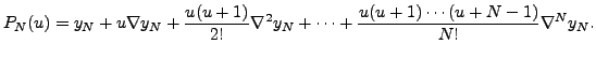
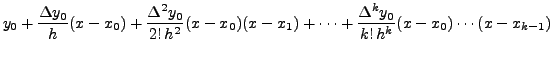
where the polynomial
So, for ![]() substitute
substitute  in (11.4.1) to get
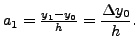
![]() This gives us
This gives us ![]() Next,
Next,
So,
 For
For
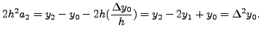
Thus,
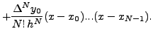
 Now, using mathematical induction, we get
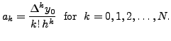
Thus,
 |
|||
 |
 and
and
and in general,
For the sake of numerical calculations, we give below a convenient form of the forward interpolation formula.
Let
![]() then
then
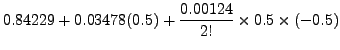
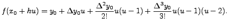
With this transformation the above forward interpolation formula is simplified to the following form:
If ![]() =1, we have a linear interpolation given by
=1, we have a linear interpolation given by
| (11.4.3) |
![$\displaystyle f(u) \approx y_0+ {\Delta y_0}(u)+\frac{\Delta ^2 y_0}{2!}[u(u-1)]$](img5079.png) |
(11.4.4) |
It may be pointed out here that if ![]() is a polynomial function
of degree
is a polynomial function
of degree ![]() then
then ![]() coincides with
coincides with ![]() on the
given interval. Otherwise, this gives only an approximation to
the true values of
on the
given interval. Otherwise, this gives only an approximation to
the true values of ![]()
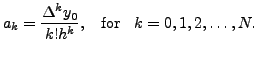
If we are given additional point ![]() also, then the error,
denoted by
also, then the error,
denoted by
![]() is estimated by
is estimated by
Similarly, if we assume, ![]() is of the form
is of the form
then using the fact that
 |
|||
 |
|||
 |
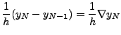
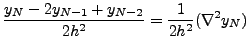
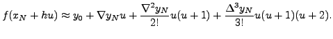
Thus, using backward differences and the transformation
![]() we obtain the Newton's backward interpolation formula as
follows:
we obtain the Newton's backward interpolation formula as
follows:
| x | 0 | 0.001 | 0.002 | 0.003 | 0.004 | 0.005 |
| y | 1.121 | 1.123 | 1.1255 | 1.127 | 1.128 | 1.1285 |
|
|
|
|
|
|
|||
| 0 | 1.121 | 0.002 | 0.0005 | -0.0015 | 0.002 | -.0025 | |
| .001 | 1.123 | 0.0025 | -0.0010 | 0.0005 | -0.0005 | ||
| .002 | 1.1255 | 0.0015 | -0.0005 | 0.0 | |||
| .003 | 1.127 | 0.001 | -0.0005 | ||||
| .004 | 1.128 | 0.0005 | |||||
| .005 | 1.1285 |
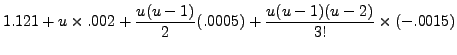
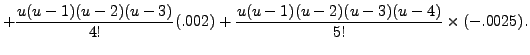
Thus, for
![]() where
where
![]() and
and
![]() we get
we get
 |
|||
 |
 |
|||
 |
|||
| 0.70 | 72 | 0.74 | 0.76 | 0.78 | ||
| 0.84229 | 0.87707 | 0.91309 | 0.95045 | 0.98926 |
|
|
|
|
|
||||
| 0.70 | 0.84229 | 0.03478 | 0.00124 | 0.0001 | 0.00001 | ||
| 0.72 | 0.87707 | 0.03602 | 0.00134 | 0.00011 | |||
| 0.74 | 0.91309 | 0.03736 | 0.00145 | ||||
| 0.76 | 0.95045 | 0.03881 | |||||
| 0.78 | 0.98926 |
In the above table, we note that
![]() is almost constant, so we
shall attempt
is almost constant, so we
shall attempt
![]() degree polynomial interpolation.
degree polynomial interpolation.
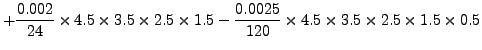
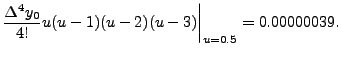
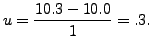
Note that
![]() gives
gives
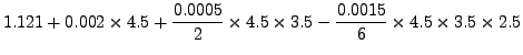
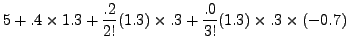
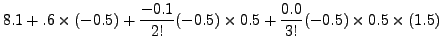
 Thus, using
forward interpolating polynomial of degree
Thus, using
forward interpolating polynomial of degree  we get

 |
 |
||
 |
|||
 |
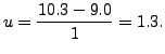
Note that exact value of
Also, find approximate value of
Therefore,
 This gives,
 |
|||
 This gives,
 |
|||
 |
 we may expect estimate calculated using
 to be a better approximation.
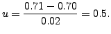
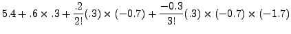
Therefore, taking
 we have
 This gives,
 |
|||
| x | 0 | 0.2 | 0.4 | 0.6 | 0.8 | 1.0 |
| y | 1.0 | 0.808 | 0.664 | 0.616 | 0.712 | 1.0 |
Compute the value of the function at ![]() and
and ![]()
| x | 0 | 50 | 100 | 150 | 200 | 250 |
| v(x) | 0 | 60 | 80 | 110 | 90 | 0 |
Find the approximate speed of the train at the mid point between the two stations.
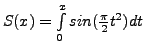 at
the different values of the tabular points
at
the different values of the tabular points
| x | 0 | 0.04 | 0.08 | 0.12 | 0.16 | 0.20 |
| S(x) | 0 | 0.00003 | 0.00026 | 0.00090 | 0.00214 | 0.00419 |
Obtain a fifth degree interpolating polynomial for ![]() Compute
Compute
![]() and also find an error estimate for it.
and also find an error estimate for it.
| Time | 8 am | 12 noon | 4 pm | 8pm |
| Temperature | 30 | 37 | 43 | 38 |
Obtain Newton's backward interpolating polynomial of degree ![]() to
compute the temperature in Kanpur on that day at 5.00 pm.
to
compute the temperature in Kanpur on that day at 5.00 pm.
![$\displaystyle y_0+\frac{\Delta y_0}{h}(h u)+\frac{\Delta^2
y_0}{2! \,h^2}\{(h u...
... \cdots + \frac{\Delta^k y_0 h^k}{k!
\, h^k} \bigl[ u(u-1)\cdots (u-k+1) \bigr]$](img5073.png)
![$\displaystyle + \cdots +\frac{\Delta ^N y_0}{N! \, h^N}
\biggl[(h u) \bigl(h(u-1) \bigr)\cdots \bigl(h(u-N+1)\bigr) \biggr].$](img5074.png)
![$\displaystyle y_0+ {\Delta y_0}(u)+\frac{\Delta ^2
y_0}{2!}(u(u-1)) + \cdots + \frac{\Delta ^k y_0}{k! }
\biggl[ u(u-1)\cdots(u-k+1) \biggr]$](img5075.png)
![$\displaystyle + \cdots +\frac{\Delta ^N y_0}{N! } \biggl[ u(u-1)...(u-N+1) \biggr].$](img5076.png)