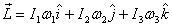
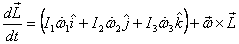
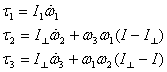
The general equation governing rotation of a rigid body:
Having dealt with situations where components of are constant, we now ask what happens when is also changed. For this let me look at the expression for the angular momentum in the principal axis frame again. It is

I now give a slightly different derivation for the rate of change of . In doing this derivation I keep in mind that as a rigid body rotates, the unit vectors along its principal axes also rotate and their rate of change is (see previous lecture)

Now I differentiate to get

Here the first term is due to the change in the components of along the principal axis and the second term is the change in due to its rotation. Notice that we recover the formula derived earlier if the components of do not change with time, i.e. . Let me repeat the interpretation of the equation: at any instant we take the body rotating in the principal axes frame at that time, i.e. the frame is frozen at its position at that time and the body is taken to be rotating in it. To see this geometrically, let me take a two-dimensional case. Shown in figure 10 are the principal axes 1 and 2 of a rigid body at times t and (t+ Δt) . In time interval Δt the body and the frame attached to it rotate by an angle , and ω₁ and ω₂ change to ω₁ + Δω₁ and ω₂ + Δω₂ . With these changes let me calculate changes in the components L₁ and L₂ in the frame frozen at time t .

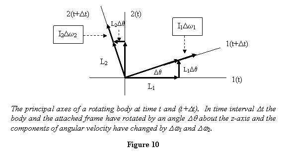
Looking at the figure, where I have shown all the changes that have taken place during the time interval Δt , we get in the frame at time t

and

So the total change in the angular momentum is

Dividing both sides by Δt and taking proper limit gives

This gives you some idea about where this equation comes from. Of course in a more accurate treatment, rotations about the other axes also have to be taken into account. For infinitesimal rotations, they can all be added up and give the general equation

This gives

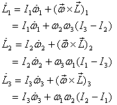
Each one of these rates of change should be equal to the component of the torque in that direction .Thus

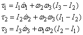
These are the most general equations governing the dynamics of a rigid body and are known as Euler's equations. I now use it to explain the third experiment I had suggested in the beginning of Lecture 21.

Example 4: Hold a rectangular box at a height with one of its faces perpendicular to the vertical, give it a spin and let it drop (see figure 11). Describe its subsequent rotational motion.

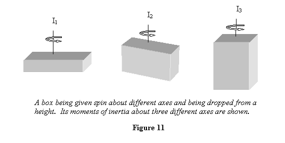
This is an example of torque-free () motion because there is no torque on the box about its centre of mass. Thus its rotational motion is governed by the equations

For a box similar to the one shown in figure 11 we would generally have I₃ > I₂ > I₁ .

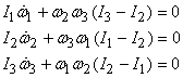
Let me first consider the case when the box is given a spin about its principal axis 1. Let me also assume that in the process I also disturb it and give it very small angular velocities ω₂ and ω₃ about its axes 2 and 3, respectively. Since both ω₂ and ω₃ are very small, their product is second-order in smallness and will be ignored. The Euler equations and there are then as given below.

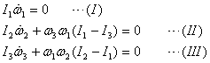
The first equation implies that ω₁ is a constant. Let me call it the spin rate ω₀ . Using this fact the other two equations are dealt with as follows. Differentiate equation (II) with respect to time to get

and substitute for from equation (III) to obtain

Since I₃ > I₂ > I₁ , the equation above is of the form

Its solution is of the form

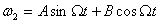
One can similarly get equation for ω₃ also and see that it also has similar oscillatory solution. This implies that as the box falls down it spins about axis 1 and oscillates about axes 2 and 3. Since magnitudes of ω₂ and ω₃ are small, you see the box fall essentially spinning only. The same thing will happen if we give initial spin about axis 3. However something different happens when the initial spin is about axis 2. Assuming ω₁ and ω₃ to be small, in this case the Euler equations take the following form right after the release of the box.

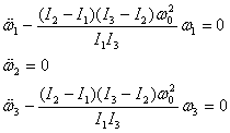
The second equation above implies that ω₂ is a constant and with I₃ > I₂ > I₁ , the other two equations take the form

Solution of these equations is of the form

which indicates that right after the release, the angular velocities about axes 1 and 3 will grow very fast and take on a large value. Thus the box will start rotating about all three axes and that is what you observe. Thus we see that a rigid body is stable when it is given a spin about the axes having the smallest or the largest moment of inertia. However, if given a spin about the axis with intermediate moment of inertia, it will be unstable. Next I take up the case of precessing top that I had not solved by employing Euler's equations earlier. This is an example where a torque is also being applied on the system

Example 5: Apply Euler's equations to a precessing top and get its precession frequency Ω. The top has a mass m and is spinning at a rate of ω_S (see figure 12). Its centre of gravity is at a distance l from the pivot point.

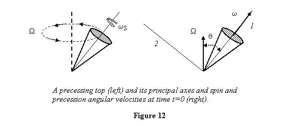
I have already discussed about the principal axes of the top in example 2 above. With the Euler's equations for the top are

Now in applying Euler's equations you have to keep in mind that the top is spinning. As such its principle axes 2 and 3 also rotate about axis 1 with angular frequency ω_S . So the components of angular frequency and torque in the direction of these axes also change with time. Taking time at which the position of the top is shown in figure 12 to be t = 0, I draw in figure 13 the position of axes 2 and 3 at time t . In this figure, I have neglected the angle W t through which the top and therefore the torque vector itself has rotated. In other words I have assumed that . Thus the angular velocity and torque are shown where they were at t = 0 .

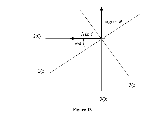
Looking at figure 13, it is clear that the components of the angular velocity and the torque are

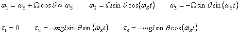
Substituting these in the Euler's equation for the top gives

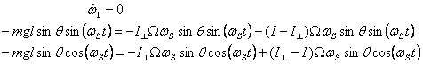
The first of these equations gives ω₁ = constant = ω_S. The other two equations give the same answer which is

This is the answer that we have seen earlier. In solving the Euler's equations for the top, we made the assumption of . Further we assumed that the top only precesses about the vertical. However, there is no reason why it cannot posses a horizontal angular velocity Ω_H also. Assuming the existence of Ω and Ω_H and then solving the Euler's equations will give a more complete solution for the motion of a spinning top. It in fact gives the nutating motion also. You may want to try getting this general solution.

With this lecture I end of the topic of rigid-body rotation.