Let us start with the example of a mass on a straight wire (say in x direction). The constraint that the mass moves only in the x-direction is equivalent to saying that

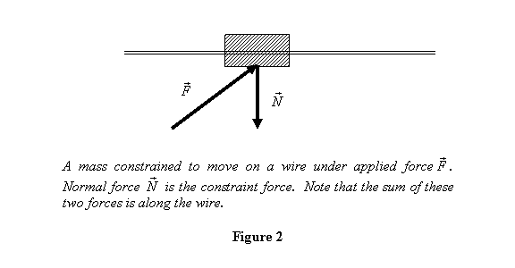
This is how we mathematically express the constraint that the mass moves only along the x-axis. As pointed out earlier, to keep the y and the z coordinates of the mass unchanged, the wire applied a normal force on the mass to cancel the perpendicular (to the wire) component of the applied force so that the net force is along the wire. This normal reaction is the constraint force (figure 2). Notice that all that the wire does to the mass, as far as its motion is concerned, is represented by this force.

.

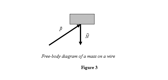
To study the motion of the mass all I need to look at are only the forces – external and constraint forces - acting on the mass. In this case the wire is represented by the normal force that it applies. Recall from lecture 4 that such a diagram is called a free-body diagram . The advantage of drawing a free-body diagram is that it identifies the relevant quantities to write the equation of motion. In the present case the free-body diagram of the mass is given in figure 3.

Let us now write the equations of motion for the body in terms of its x, y and z -components :

Let us count how many unknown are there? The unknowns are x , y , z , N_y , and N_z , numbering five (is given). But there are only three equations. How do we find the other two equations? For this recall that the two of the unknowns, N_x and N_y , arise because of the constraints. And it is these constraints that provide the two more equations needed for a solution. The constraints that y = constant and z = constant imply that

With these two additional equations, we now have five equations and five unknowns. Thus and we can solve for x , y , z and N_x and N_y in terms of given parameters of the problem.

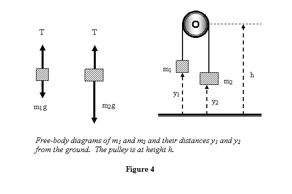
Let us now look at the other problem of two masses hanging on the sides of a frictionless pulley (see figure 1), a special case of Atwood's Machine. For simplicity we take the pulley and the rope to be massless. Let the masses be m₁ & m₂ . In this problem also the motion is in only one direction i.e. the vertical direction so we are going to ignore the other two dimensions. In this problem the constraint is that the two masses move together and it is effected by the rope. As noted above, the force of constraint therefore is the tension T in the rope. Let us now make their free-body diagrams for the two moving masses m₁ and m₂. We measure all distances from the ground and let the distance of m₁ be y₁ and that of m₂ is y₂ . Please see figure 4.

Equation of motion for m₁ and m₂ are

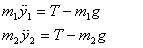
The tension T is the same on both sides because rope and pulley both are massless and the pulley is also frictionless. These are two equations and there are three unknowns: y₁ , y₂ and T . The tension T arises because of constraint so the constraint itself provides the desired third equation. In this case the constraint is that the length of the rope is constant. This can be expressed mathematically as (see figure 4 for meaning of symbols)

where R is the radius of the pulley. Differentiating this equation twice with respect to time gives

We now have three equations for three unknowns:

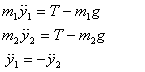
Solving these equations gives

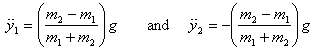
a result that you already know. Thus if m₂ >m₁, m₁ accelerates up.

Through these two simple examples, I have identified sequential steps that we take in solving a problem involving constraints I now summarize these steps:

1. Identify the constraints and forces of constraints in the given problem;
2. Make free body diagrams of different bodies taking part in the motion. Let me remind you in making free body diagram take the body and show all the forces - applied and those of constraints - on the body;
3. Write equations of motion for each subsystem/body. At this stage the number of equations will be less than the number of variables in the problem;
4. Write the constraint equations. They will provide the missing equations (This happens because each constraint introduces a constraint force which becomes the additional unknown);
5. Solve the equations.