Lecture 10
Method of Virtual Work

So far when dealing with equilibrium of bodies/trusses etcetera, our strategy has been to isolate parts of the system (subsystem) and consider equilibrium of each subsystem under various forces: the forces that we apply on the system and those that the surfaces, and other elements of the system apply on the subsystem. As the system size grows, the number of subsystems and the forces on them becomes very large. The question is can we just focus on the force applied to get it directly rather than going through each and every subsystem. The method of virtual work provides such a scheme. In this lecture, I will give you a basic introduction to this method and solve some examples by applying this method.

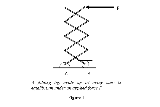
Let us take an example: You must have seen a children's toy as shown in figure 1. It is made of many identical bars connected with each other as shown in the figure. One of the lowest bars is connected to a fixed pin joint A whereas the other bar is on a pin joint B that can move horizontally. It is seen that if the toy is extended vertically, it collapses under its own weight. The question is what horizontal force F should we apply at its upper end so that the structure does not collapse.

To see how many equations do we have to solve in finding F in the structure above, let us take a simple version of it, made up of only two bars, and ask how much force F do we need to keep it in equilibrium (see figure 2).

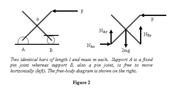
Let each bar be of length l and mass m and let the angle between them be θ. The free-body diagram of the whole system is shown above. Notice that there are four unknowns - N_Ax , N_Ay , N_By and F - but only three equilibrium equations: the force equations

and the torque equation

So to solve for the forces we will have to look at individual bars. If we look at individual bars, we also have to take into account the forces that the pin joining them applies on the bars. This introduces two more unknowns N₁ and N₂ into the problem (see figure 3). However, there are three equations for each bar - or equivalently three equations above and three equations for one of the bars - so that the total number of equations is also six. Thus we can get all the forces on the system.

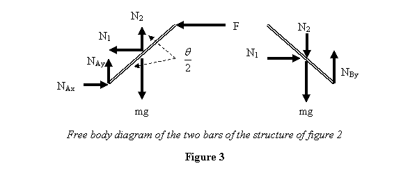
The free-body diagrams of the two bars are shown in figure 3. To get three more equations, in addition to the three above, we can consider equilibrium of any of the two bars. In the present case, doing this for the bar pinned at B appears to be easy so we will consider that bar. The force equations for this bar give

And taking torque about B , taking N₁ = 0 , gives

This then leads to (from the force equation above)

Substituting these in the three equilibrium equations obtained for the entire system gives

Looking at the answers carefully reveals that all we are doing by applying the force F is to make sure that the bar at pin-joint A is in equilibrium. This bar then keeps the bar at joint B in equilibrium by applying on it a force equal to its weight at its centre of gravity.

The question that arises is if we have many of these bars in a folding toy shown in figure 1, how would we calculate F ? This is where the method of virtual work, to be developed in this lecture, would come in handy. We will solve this problem later using the method of virtual work. So let us now describe the method. First we introduce the terminology to be employed in this method.

1. Degrees of freedom: This is the number of parameters required to describe the system. For example a free particle has three degrees of freedom because we require x, y , and z to describe its position. On the other hand if it is restricted to move in a plane, its degrees of freedom an only two. In the mechanism that we considered above, there is only one degree of freedom because angle θ between the bars is sufficient to describe the system. Degrees of freedom are reduced by the constraints that are put on the possible motion of a system. These are discussed below.

2. Constraints and constraint forces: Constraints and those conditions that we put on the movement of a system so that its motion gets restricted. In other words, a constraint reduces the degrees of freedom of a system. Constraint forces are the forces that are applied on a system to enforce a constraint. Let us understand these concepts through some examples.

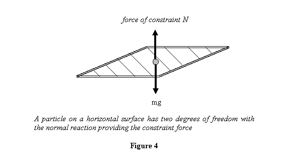
A particle in free space has three degrees of freedom. However, if we put it on a plane horizontal surface without applying any force in the vertical direction, its motion is restricted to that plane. Thus now it has only two degrees of freedom. So the constraint in this case is that the particle moves on the horizontal surface only. The corresponding force of constraint is the normal reaction provided by the surface.

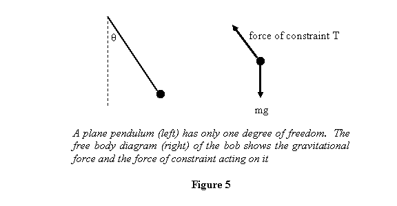
As the second example, let us take the case of a vertical pendulum oscillating in a plane (see figure 5). Thus its degrees of freedom would be two if there were no more constraints on its motion. However, the bob of a pendulum is constrained to move in such a way that its distance from the pivot point remains fixed. We have thus introduced one more constraint on its motion and therefore the degrees of freedom are reduced by one; a pendulum oscillating in a plane has only one degree of freedom. The angle from the equilibrium position is therefore sufficient to describe a plane pendulum's motion fully. How about the force of constraint in this case? The constraint, that the distance of the bob from the pivot point remains fixed, is ensured by the tension in the string. The tension in the string is therefore the force of constraint.

Let us now consider the folding toy shown in figure 1. This structure, although made of many moving bars, has only one degree of freedom because the bars are constrained to move in a very specific way. Thus from a large number of degrees of freedom for these bars, all of them except one are eliminated by the constraints. As such the number of constraints, and therefore the number of constraint forces, is very large. The constraint forces are the reactions at the supports A and B and the forces applied by the pins holding the bars together. It is because of these forces that the system is restricted in its motion.

I would like you to note one thing interesting in the examples considered above: if the system moves the constraint forces do not do any work on it. In the case of a particle moving on a plane, the motion is perpendicular to the normal reaction so it does no work on the particle. In the pendulum the motion of the bob is also perpendicular to the tension in the string which is the force of constraint. Thus no work is done on the bob by the constraint force. The case of the toy in figure 1 is quite interesting. In the structure point A does not move and the motion of point B is perpendicular to the reaction force at B. Thus there is no work done by the reaction forces at these points. On the other hand, the constraint forces due to pins connecting two bars are equal and opposite on each bar. But the points on the bar where these forces act (the points where the pin joints are) have the same displacement for each bar so that the net work done by the constraint forces vanishes.

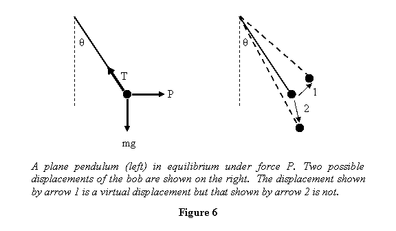
3. Virtual displacement: Given a system in equilibrium, its virtual displacement is imagined as follows: Move the system slightly away from its equilibrium position arbitrarily but consistent with the constraints. This represents a virtual displacement of the system. Note the emphasis on the word imagined. This is because a virtual displacement is not caused by the applied forces. Rather it is the difference between the equilibrium position of the system and an imagined position - consistent with the constraints - of the system slightly away from the equilibrium. For example in the case of a pendulum under equilibrium at an angle θ under a force P (see figure 6), virtual displacement would be increasing the angle from θ to ( θ + Δθ) keeping the distance of the bob from the pivot unchanged. On the other hand, moving the bob with a component in the direction of the string is not a virtual displacement because it will not be consistent with the constraint. Virtual displacement is denoted by to distinguish it from a real displacement .

4. Virtual work: The work done by any force during a virtual displacement is called virtual work. It is denoted by . Thus

Note that our previous observation, that work done by a constraint force is usually zero, implies that virtual work done by a constraint force is also zero. Also keep in mind that in calculating the work done by the force , represents the displacement of the point where the force is being applied.

With these definitions we are now ready to state the principle of virtual work. It is based on the assumption that virtual work done by a constraint force is zero. The principle of virtual work states that " The necessary and sufficient condition for equilibrium of a mechanical system without friction is that the virtual work done by the externally applied forces is zero ". Let us see how it arises. For a system in equilibrium, each particle in the system is in equilibrium under the influence of externally applied forces and the forces of constraints. Then for the i^th particle

Therefore

But we have already seen that for individual particles and for a system composed of many subsystems , that is the net virtual work done by constraint forces is zero. This means that the total virtual work done by the external forces vanishes, i.e.

This is the necessary part of the proof. The condition is also sufficient condition. This is proved by showing that if the body is not in equilibrium, the virtual work done by the external forces does not vanish for all arbitrary virtual displacements (consistent with the constraints). If the body is not in equilibrium, it will move in the direction of the net force on each particle. During this real displacement the work don by the force on the i^th particle will be positive i.e.

Now we can choose this real displacement to be the virtual displacement and find that when the body is not in equilibrium, all virtual displacements consistent with the constraints will not give zero virtual work. Thus when the system is not in equilibrium

Assuming again that the net work done by the constraint forces is zero, we get that for a body not in equilibrium

This implies that when the virtual work done by external forces vanishes, the system must be in equilibrium. This proves the sufficiency part of the condition. We now solve some examples to illustrate how the method of virtual work is applied.