Low pass filter with adjustable corner frequency

One advantage of active filter is that it is often quite simple to vary parameter values. As an example, a first-order low-pass filter with adjustable corner frequency is shown in fig. 3.

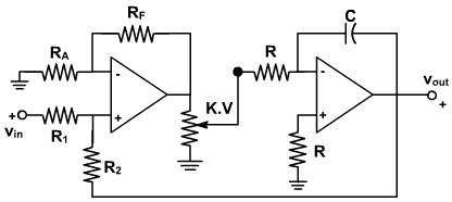
Fig. 3

The voltage at the opamp inputs are given by

Setting v + = v -, we obtain the voltage, v₁, as follows:

where

The second opamp acts as an inverting integrator, and

Note that we use upper case letters for the voltages since these are functions of s. K is the fraction of V₁ sent to the integrator. That is, it is the potentiometer ratio, which is a number between 0 and 1.

The transfer function is given by

The dc gain is found by setting s = 0 (i.e., jω =0)

The corner frequency is at KA₂ / RC. Thus, the frequency is adjustable and is proportional to K. Without use of the opamp, we would normally have a corner frequency which is inversely propostional to the resistor value. With a frequency proportional to K, we can use a linear taper potentiometer. The frequency is then linearly proportional to the setting of the potentiometer.

Example - 2

Design a first order adjustable low-pass filter with a dc gain of 10 and a corner frequency adjustable from near 0 t0 1 KHz.

Solution:

There are six unknowns in this problems (RA, RF, R1, R2, R and C) and only three equations (gain, frequency and bias balance). This leaves three parameters open to choice. Suppose we choose the following values:

C = 0.1 µF
R = 10 KΩ
R₁ = 10KΩ

The ratio of R₂ to R₁ is the dc gain, so with a given value of R₁ = 10KΩ, R₂ must be 100 kΩ. We solve for A₁ and A₂ in the order to find the ratio, R_F / R_A.

The maximum corner frequency occurs at K = 1, so this frequency is set to 2π x 1000. Since R and C are known, we find A₂ = 6.28. Since A₂ and A₁ are related by the dc gain, we determine A₁ / A₂ = 10 and A₁ = 62.8. Now, substituting the expression for A₂, we find

and since

we find R_F / R_A = 68. R_A is chosen to achieve bias balance. The impedance attached to the non-inverting input is 10 KΩ || 100 KΩ = 10 KΩ.

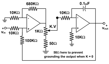
Fig. 4

If we assume that R_F is large compared with R_A ( we can check this assumption after solving for these resistors), the parallel combination will be close to the value of R_A. We therefore can choose R_A = 10 KΩ. With this choice of R_A, R_F is found to be 680KΩ and bias balance is achieved. The complete filter is shwn in fig. 4.

GOTO >> 1 || 2 || 3 || Home