| |
Arbitrary input signals:
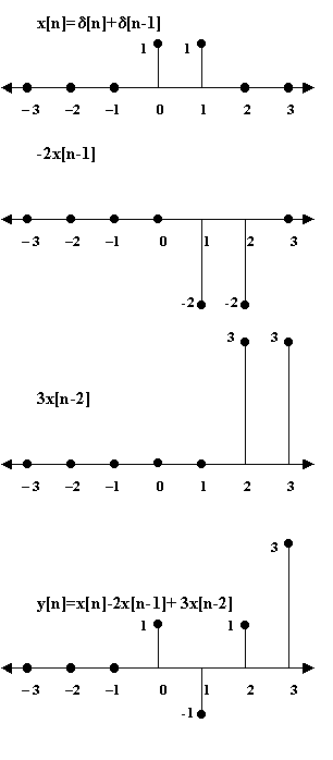
Now let us consider some other input, say x[0]=1, x[1]=1 and x=0 for n other than 0 and 1. What will be the response of the above LSI system to this input? We calculate the response in a table as below
|
y[n] = x[n] - 2x[n-1] + 3x[n-2] |
x[n]= + +
 |
|
n |
y1[n] from
 |
y2[n] from - |
y[n] = y1[n] + y2[n] |
|
..., -1 |
0 |
0 |
0 |
|
0 |
1 |
0 |
1 |
|
1 |
-2 |
1 |
-1 |
|
2 |
3 |
-2 |
1 |
|
3 |
0 |
3 |
3 |
|
4, ... |
0 |
0 |
0 |
Ah! What we have actually done, is applied the additive (linear), homogenous (linear) and shift invariance properties of the system to get the output. First, we decomposed the input signal as a sum of known signals: first being the unit step
. The second signal is derived from the unit step by shifting it by
1. Thus, our input signal is as shown in the figure below. Then, we invoke the LSI properties of the system to get the responses to the individual signals: the first calculation is show above, while the calculation of response for
is shown below.
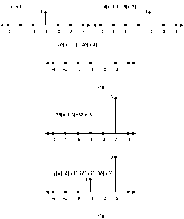
Finally, we add the two responses to get the response
y[n] of the system to the input x[n]. The image below shows the final response with an alternative method of calculating it:
This brings us up to the concept of convolutions, covered in detail in a later section. 
|