Example Related to Discrete Time LTI Systems

Recall that the convolution sum is given by

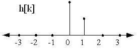
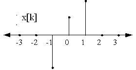
Now we plot x[k] and h[n-k] as functions of k and not n because of the summation over k. Functions x[k] and h[k] are the same as x[n] and h[n] but plotted as functions of k. Then, the convolution sum is realized as follows

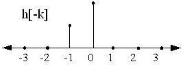
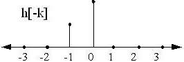
1. Invert h[k] about k=0 to obtain h[-k].

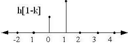
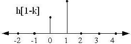
2. The function h[n-k] is given by h[-k] shifted to the right by n (if n is positive) and to the left (if n is negative). It may appear contradictory but think a while to verify this (note the sign of the independent variable).

In the figure below n=1

3. Multiply x[k] and h[n-k] for same coordinates on the k axis. The value obtained is the response at n i.e. Value of y[n] at a particular n the value chosen in step 2. Now we demonstrate the entire procedure taking n=0,1 thereby obtaining the response at n=0,1. The input signal x[n] and for this example is taken as : 

Case 1: For n=0

Remember the independence axis has k as the independent variable. Then taking the product x[k] h[-k] for same k and summing it we get the value of the response at n=0.

Let h[-k] = g[k]

y[0] = ...........x[-1]g[-1] + x[0] g[0] +............... = (-2) (1) +(1) (2) = 0

Case 2: For n=1

h[1-k] =g[k]

y[1] = .........+ x[0]g[0] + x[1]g[1] + ............. = (1)(1) +(2)(2) = 5

The values are the same as that obtained previously.  

The total response referred to as the Convolution sum need not always be found graphically. The formula can directly be applied if the input and the impulse response are some mathematical functions. We show this by an example next.