Substituting s in the above equation we get:
2.gif)
Observing the above
equation closely, we realize that firstly H(s) converges if
and only if
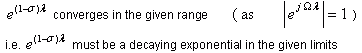
We analyze the part (1-σ)
as follows:
 For a decaying e(1-σ)λ
it
is essential that (1-
For a decaying e(1-σ)λ
it
is essential that (1- )< 0
. This implies that (> 1)
which means that the Real part of 's' is greater than '1'
which is also denoted as Re(s) > 1.
)< 0
. This implies that (> 1)
which means that the Real part of 's' is greater than '1'
which is also denoted as Re(s) > 1.
This is what
defines the " Region of Convergence " in
an S-Complex Plane. The ROC of the
Laplace Transform is always determined by the Re(s).
The ROC in general gives us an idea
of the stability of a system and is also a
representation of the poles-zero plot of a system.
It is
essential to note that the ROC never includes poles.
Evaluation of the
integral yields:
H(s)=4.gif) =1/(s-1)
=1/(s-1)
We observe that there
is a single pole at s=1. Since the Region of
Convergence cannot contain
poles therefore ROC start from '1' and tends outwards to
infinity.
est
in physical systems:
We
consider the real part of est,
where s = σ + jΩ
.
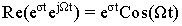
Such a response is visible in
RLC (Resistance-Inductance and Capacitance)
systems. It is
not only visible in the electrical field but also in other disciplines like mechanical field.
In such
cases the above expression is multiplied by a polynomial or a combination of such expressions.
1.gif)