
Contents
Theory behind the Application
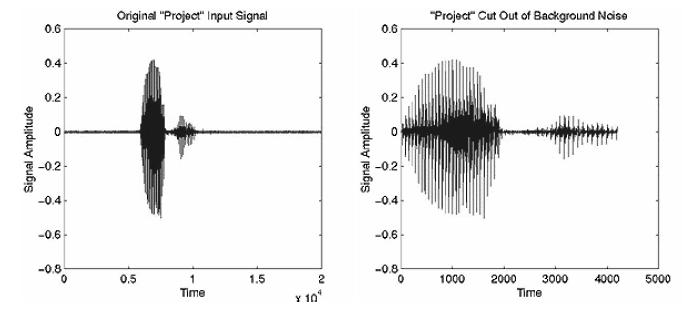
5.1 Endpoint Detection
The endpoint detection algorithm functions as follows:1) The process removes any DC offset in the signal. This is a very important step because the zero-crossing rate of the signal is calculated and plays a role in determining where unvoiced sections of speech exist. If the DC offset is not removed, we will be unable to find the zero-crossing rate of noise in order to eliminate it from our signal.
2) Compute the average magnitude and zero-crossing rate of the signal as well as the average magnitude and zero-crossing rate of background noise. The average magnitude and zero-crossing rate of the noise is taken from the first hundred milliseconds of the signal. The means and standard deviations of both the average magnitude and zero-crossing rate of noise are calculated, enabling us to determine thresholds for each to separate the actual speech signal from the background noise.
3) At the beginning of the signal, we search for the first point where the signal magnitude exceeds the previously set threshold for the average magnitude. This location marks the beginning of the voiced section of the speech.
4) From this point, search backwards until the magnitude drops below a lower magnitude threshold.
5) From here, we search the previous twenty-five frames of the signal to locate if and when a point exists where the zero-crossing rate drops below the previously set threshold. This point, if it is found, demonstrates that the speech begins with an unvoiced sound and allows the algorithm to return a starting point for the speech, which includes any unvoiced section at the start of the phrase.
6) The above process will be repeated for the end of the speech signal to locate an endpoint for the speech.
5.2 Dynamic Time Warping
The end result of the short time magnitude and short time frequency is a new, time-varying sequence that serves as a new representation of the speech signal. Suppose in the fig.1 the two signals are the new representation of the input signal and the key signal. As we can see from the fig.1 the appropriate sections on the two signals are not aligned as the second lobe of the input signal is bit delayed compared to the second lobe of the key signal. In such a situation comparison of the two signals will yield poor results. Now if the above two signals are processed through Dynamic Time Warping (DTW), it non-linearly maps one of the two signals onto the other by minimizing the distance between the two signals. Hence the two signals have all their appropriate sections aligned as shown in the fig 2. On comparison of these newly mapped signals will yield far better results than before.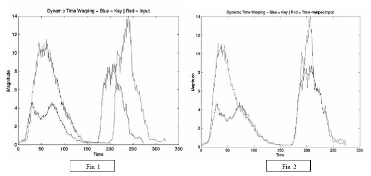
5.3 Feature Extraction
5.3.1 Short-Time Magnitude
The short-time magnitude characterizes the envelope of a speech signal by lowpass filtering it with a rectangular window. The magnitude function follows these steps: The bounds of the signal are determined and each end is zero-padded. The signal is convolved with a rectangular window. As the window is swept across the signal, the magnitude of the signal contained within it is summed and plotted at the midpoint of the windows location. One magnitude plot is discrete time warped onto the other. The dot product of the two waveforms is computed, and this number is divided by the product of the signals norms as mandated by the Cauchy- Schwarz Inequality. This calculation results in a percentage of how similar one signal is to the other.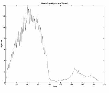
5.3.2 Short-Time Frequency
To extract pitch from our signals, we make use of a harmonic-peak-based method. Since harmonic peaks occur at integer multiples of the pitch frequency, we can compare peak frequencies at each time t to locate the fundamental. Our implementation finds the three highest-magnitude peaks for each time. Then we compute the differences between them. Since the peaks should be found at multiples of the fundamental, we know that their differences should represent multiples as well. Thus, the differences should be integer multiples of one another. Using the differences, we can derive our estimate for the fundamental frequency. Derivation:Let f1 = lowest-frequency high-magnitude peak
Let f2 = middle-frequency high-magnitude peak
Let f3 = highest-frequency high-magnitude peak
Then d1 = f2-f1 and d2 = f3-f2.
Assuming that d2 > d1, let n = d2/d1. Then our estimate for the fundamental frequency is F0 = (d1+d2) / (n+1).
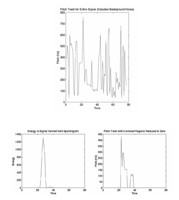
We find the pitch frequency at each time and this gives us our pitch track. A major advantage to this method is that it is very noise-resistive. Even as noise increases, the peak frequencies should still be detectable above the noise. In order to do this,
We first find the signal's spectrogram. We assume that the fundamental frequency (pitch) of any person's voice will be at or below 1200 Hz, so when finding the three largest peaks, we only want to consider sub- 1200 Hz frequencies. Thus, we want to cut out the rest of the spectrogram. Before we do this, however, we must use the whole spectrogram to find the signal's energy. The signal's energy at each time shows the voiced and unvoiced areas of the signal, with voiced areas having the higher energies. Since we are using our pitch track to compare pitch between signals, we want to be certain that we are only comparing the voiced portions, as they are the areas where pitch will be distinct between two different people. A plot of energy versus time can actually be used to window our pitch track, so that we may get only the voiced portions. To find the energy versus time window, we take the absolute magnitude of the spectrogram and then square it. By Parseval's Theorem, we know that adding up the squares of the frequencies at each time gives us the energy of the signal there. Plotting this versus time gives us our window. Once this is done, we cut our spectrogram and move on to finding the three largest peaks at each time. This is done by observing the peaks on the new edited spectrogram. When the three largest peaks at each time are known , the fundamental frequency at each time is calculated using the above derived mathematical expressions. The graph of the pitch track of only the voiced region is obtained from these fundamental frequencies.