

Contents
A PCM recorder
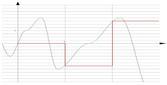
In the following figures the red lines are the values of the output under a zero-order hold
approximation that is the value is retained until the next sampling point in time comes in.
(note that the mechanism responsible for the hold is not a part of our system but is
depicted here to make understanding the system easy)
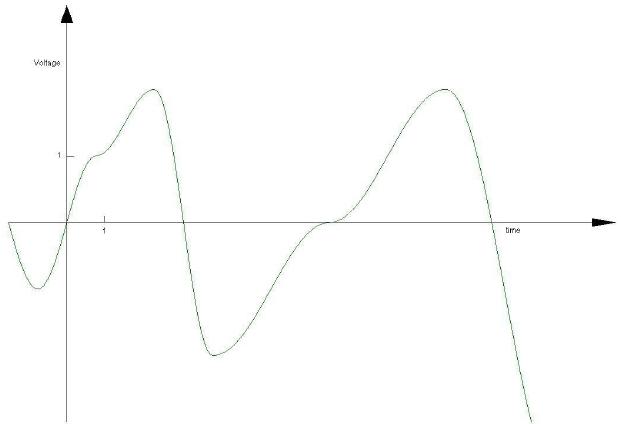
Some of the sampled waveforms are redrawn below.
Let sampling rate and bit depth be say once every 4*n units and bit-depth be
m digits respectively for the following sampled output.
In the following figure the values for sampling rate and bit-depth would be n and m-1
digits respectively.
In the following figure the values for sampling rate and bit-depth would be n and m+1
digits respectively.
In the following figure the values for sampling rate and bit-depth would be n and m+1
digits respectively.
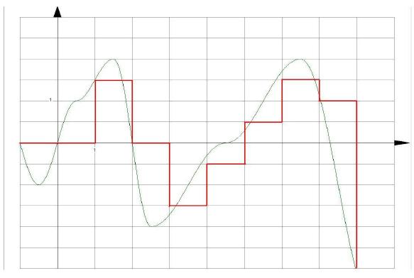
As we observe higher sampling frequencies result in better approximations of the original
signal. And as mentioned, let us say the human ear in this example cant differentiate
between two sounds if they are less than 2*n unit Hz apart (while having the same
intensity) and less than 2^m units apart in intensity. Then as we notice there is no need
for sampling at frequencies higher than 2*n and for allocating more than m digits for
the bit-depth. Of course higher values than these are used to make the sound seem even
better an approximation though we really cant tell the difference.
The analog filters can only but emulate the ideal ones we are constricted to sampling at
higher frequencies since this ensures better phase (zero or linear) and magnitude (almost
constant in the region of audible frequencies) filter since they are situated close to the
origin and the response being much flatter there. Thus higher sampling frequencies are
used to obtain better quality of sound. For example, DVD has a sampling rate of 96kHz
while using 20 or 24 as the bit-dept, whereas production quality uses 192kHz giving
much better sound due to better approximations of the original signal.
The commonly used sampling rate and bit-depth is 16-bit 44.1kHz sampling used in the
.wav or .aiff file types. Though theoretically we can adjust the bit-depth and sampling rate
to be anything we wish, the only fallout being that the audio quality would be depend
accordingly. As mentioned earlier this is the input to the compression algorithms which
further manage to minimize this data (termed lossy compression as compared to lossless
compression that we are dealing with) by use of powerful and complex methods which
also manage to recover the original data without much loss as compared to the reduction
in data which they manage.
Peek into the actual algorithms : Since the data storage required for such audio is quite
high we use further compression of this data by ignoring some and representing the rest in
more concise manner. This process involves algorithms using complex mathematical
calculations with respect to intensity of sound, repetitive sound heard again and again
during a recording, variable rate of coding ( www.wavetrace.com www.mp3-tech.com
)etc which aims to minimize the data required to store a song, all driven by download (
transfer ) time taken.
Why digital audio :
Analog audio has many obvious shortcomings. For example making a copy introduces
noise and unwanted signals every time due to mechanical contact. The storage mechanism
(tapes, etc.) have limited performance and life that is undergo degradation. Analog audio
has uneven frequency response. Error correcting data cannot be added and data
lost/damaged cannot be replaced.
Besides everything nowadays is going digital, and it is the obvious choice too since it is
much longer lasting, has better performance parameters like flat audio response, higher
dynamic range (96 dB as opposed to maximum of 80 dB for analog) etc.
Besides since all technologies now use digital format of all available material it has
become inevitable too.
Playback is achieved by approximation of the sampled output using various techniques
like sample and hold technique, linear approximation, 2nd order approximation etc.
Now we look at the properties of the system under consideration. To repeat, the system
has the following inputs and output.
Audio i/p , Sampling rate, Bit-Depth :: Sampling going on at specific intervals of time,
binary digits as output.

