The above eqn. indicates that when H = 0, the magnetization points along the easy axis and when
H = H_k , the magnetization points along the direction of H . For any intermediate value of the applied field, the magnetization points at a value of angle given by eqn.(3.5) rotating smoothly between the easy axis and the applied field.

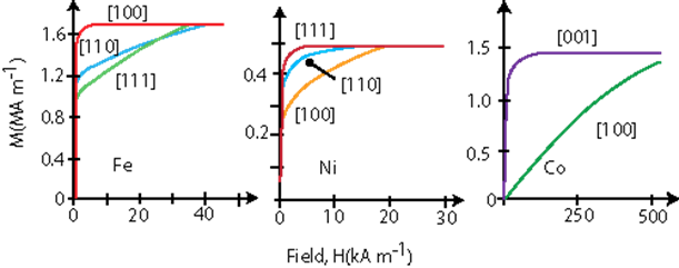
$Description: F:\NPTEL II courses\02_Phys_Mag_record\PMR_Drawn_images\fig 5.27.png$

Figure 3.2: Magnetization of single crystals of Iron, Nickel and Cobalt.

Magnetocrystalline anisotropy:

Figure 3.2 depicts the initial magnetization curves of single crystals of the different 3d ferromagnetic elements. It is clearly seen that they show a different approach to saturation when magnetized in different directions. For example, the iron shows a 〈 100 〉 as easy directions and 〈 111 〉 as hard directions, while the nickel exhibits 〈 111 〉 as easy axis and 〈 100 〉 as hard directions. This property can be understood by analysing the development of anisotropy energy in different symmetries as given below:

For Hexagonal:

For Tetragonal:

For Cubic:

(3.6)

where α_i are the direction cosines of the magnetization. The K_1c term is equivalent to . When, θ = 0, Φ = 0, this term reduces to eqn.(3.1).

Origin of magnetocrystalline anisotropy :

There are two distinct sources of magnetocrystalline anisotropy: (i) single-ion contributions and (ii) two-ion contributions. The first one is essentially due to the electrostatic interaction of the orbitals containing the magnetic electrons with the potential created at the atomic site by the rest of the crystal. This crystal field interaction stabilizes a particular orbital and by spin-orbit interaction, the magnetic moment is aligned in a particular crystallographic direction. For example, a uniaxial crystal having 2 X 10²⁸ ions/m³ , described by a spin Hamiltonian DS ² with D / k_B = 1 K and S = 2 will have anisotropy constant K 1 = nDS² = 1.1 ´ 10⁶ J/m³ .

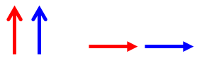
Figure 3.3: Schematic drawing of broadside and head-to-tail configurations for a pair of ferromagnetically coupled magnetic moments.

On the other hand, the later contribution replicates the anisotropy of the dipole-dipole interaction. Considering the broadside and head-to-tail configurations of two dipoles, as shown in Fig.3.3, each with moment m, the energy of the head-to-tail configuration is lower by and hence the magnets tend to align head-to-tail. In non-cubic lattices, the dipole interaction is an appreciable source of ferromagnetic anisotropy.