Let us consider a macroscopic system at thermodynamic equilibrium with a heat bath at temperature T. (Hence, we will be developing the MC technique here in the frame work of canonical ensemble.) As per statistical mechanics (discussed in chapter- 1), if the system is system is described by a Hamiltonian function H, the expectation value of a macroscopic quantity A is given by

where the canonical partition function Z is given by

whereas if system described by discrete energy state, energy corresponding to the state s, the expectation value of a macroscopic quantity A is then given by

where is the canonical partition function. Note that the partition function Z involves either evaluation of summation over all possible states, an infinite series or an integration over a 6N dimensional space. The partition function gives the exact description of a system. However, in most of the cases, it is not possible to evaluate the partition function analytically or even exactly numerically. The difficulty is not only in evaluating the integral or summation over 6N degrees of freedom but also handling the complex interaction appearing in the exponential. In general, it is not possible to evaluate the summation over such a large number of state or the integral in such a high dimensional space. On the other hand, at low temperature the system spends almost all its time sitting in the ground state or one of the lowest excited states. Thus, an extremely restricted part of the phase space should contribute to the average. Accordingly, the sum should be over a few low energy states because at low temperature there is not enough thermal energy to lift the system into the higher excited states. Thus, picking up points randomly over the phase space is no good here.

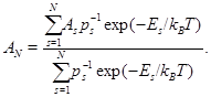
However, it is always possible to take average over a finite number of states, a subset of all possible states, if one knows the correct Boltzmann weight of the states and the probability with which they are picked up. This can be realized in MC simulation technique. In MC simulation techniques, usually only states are considered for making average. Say, N states , a small subset of all possible states, are chosen at random with certain probability distribution . So the best estimate of the physical quantity A will be

Note that the Boltzmann probability of each state is normalized by the probability of choosing the state. As the number of sample N increases, the estimate will be more and more accurate. Eventually, as , .

Now, the problem is how to specify so that the chosen N states will lead to right <A>. Depending on the nature of a physical problem, the choice of in MC averaging may differ. The physical problems can be categorized in two different groups: non-thermal non-interacting and thermal interacting systems. For non-thermal non-interacting systems `simple sampling MC' and for thermal interacting systems `importance sampling MC' are found suitable respectively.