• The boundary conditions as in Eg. (28.16), in combination with Eg. (28.21a) and (28.21b) become
  

at , therefore

• Blasius obtained the solution of this equation in the form of series expansion through analytical techniques
  
• We shall not discuss this technique. However, we shall discuss a numerical technique to solve the aforesaid equation which can be understood rather easily.
  
• Note that the equation for does not contain . 
  
• Boundary conditions at and merge into the condition . This is the key feature of similarity solution.
  
• We can rewrite Eq. (28.22) as three first order differential equations in the following way

(28.24a)

(28.24b)

(28.24c)

• Let us next consider the boundary conditions.

1. The condition remains valid.
   
2. The condition means that .
   
3. The condition  gives us .
   

Note  that the equations for f and G have initial values. However, the value for H(0) is not known. Hence, we do not have a usual initial-value problem.

Shooting Technique

We handle this problem as an initial-value problem by choosing values of and solving by numerical methods , and .

In general, the condition will not be satisfied for the function arising from the numerical solution.
We then choose other initial values of so that eventually we find an which results in .
This method is called the shooting technique .

• In Eq. (28.24), the primes refer to differentiation wrt. the similarity variable . The integration steps following Runge-Kutta method are given below.

(28.25a)

(28.25b)

(28.25c)

• One moves from to . A fourth order accuracy is preserved if h is constant along the integration path, that is, for all values of n . The values of k, l and m are as follows.
  
• For generality let the system of governing equations be

In a similar way K₃, l₃, m₃ and k₄, l₄, m₄ mare calculated following standard formulae for the Runge-Kutta integration. For example, K₃ is given by The functions F₁, F₂and F₃ are G, H , - f H / 2 respectively. Then at a distance from the wall, we have

(28.26a)

(28.26b)

(28.26c)

(28.26d)

• As it has been mentioned earlier is unknown. It must be determined such that the condition is satisfied.

The condition at infinity is usually approximated at a finite value of  (around ). The process of obtaining accurately involves iteration and may be calculated using the procedure described below.

• For this purpose, consider Fig. 28.2(a) where the solutions of versus for two different values of are plotted.
  The values of are estimated from the curves and are plotted in Fig. 28.2(b).
  
• The value of now can be calculated by finding the value at which the line 1-2 crosses the line By using similar triangles, it can be said that . By solving this, we get .
• Next we repeat the same calculation as above by using and the better of the two initial values of . Thus we get another improved value . This process may continue, that is, we use and as a pair of values to find more improved values for , and so forth. The better guess for H (0) can also be obtained by using the Newton Raphson Method. It should be always kept in mind that for each value of , the curve versus is to be examined to get the proper value of .
• The functions and are plotted in Fig. 28.3.The velocity components, u and v inside the boundary layer can be computed from Eqs (28.21a) and (28.21b) respectively.
• A sample computer program in FORTRAN follows in order to explain the solution procedure in greater detail. The program uses Runge Kutta integration together with the Newton Raphson method

Download the program

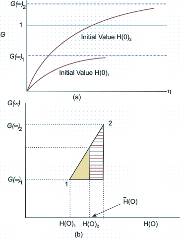  Fig 28.2     Correcting the initial guess for H(O)



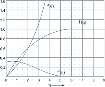Fig 28.3      f, G and H distribution in the boundary layer



• Measurements to test the accuracy of theoretical results were carried out by many scientists. In his experiments, J. Nikuradse, found excellent agreement with the theoretical results with respect to velocity distribution within the boundary layer of a stream of air on a flat plate.
• In the next slide we'll see some values of the velocity profile shape and in tabular format.