Local or Element Notation

In the last lecture, we introduced a numbering scheme for the elements, nodes, nodal coordinates and basis functions. This is called as the global numbering scheme . It is shown in Fig. 6.1.

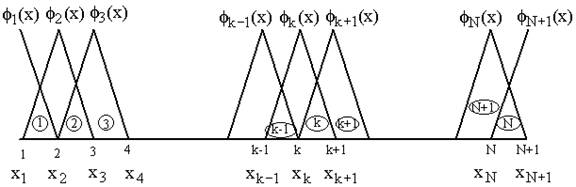
Figure 6.1 Global numbering scheme

For the convenience of the element wise evaluation of the stiffness matrix and the force vector, at the element level, we introduce another numbering scheme for the nodes, nodal coordinates and basis functions. This scheme is called as the local or element numbering scheme. For k-th element, this numbering scheme is illustrated in Fig. 6.2

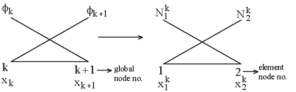
Figure 6.2 Elemental numbering scheme for k-th element

For k-th element, note that, the global numbers of the two end nodes are k and k+1 respectively (Fig. 6.1). Now we number them as 1 and 2 (Fig. 6.2). We call it as the local or element node numbering scheme . Note that the global notation for the coordinates of the end nodes is and (Fig. 6.1). Now, we denote them as and (Fig. 6.2). This is called as the local or element notation . The subscript here denotes the local node number. For every element, the nodes will always be numbered as 1 and 2 according to the local numbering scheme. Therefore to identify the element under consideration, a superscript is added to the notation of the coordinates. The superscript denotes the element number. Figure 6.1 shows that the only non-zero basis functions for the -th element are and . This is the global notation for the basis functions. Under the local or element notation , we denote them as and . Here, the subscript denotes the local number of the node at which the basis function attains the value unity and the superscript represents the element number under consideration. These functions are called as the shape or interpolating functions . Using equation (5.3), the expressions for the shape functions can be written as:

(6.1)

where the expression (5.2) for the element size becomes

=	(6.2)

Consider the expression (5.5) for the approximate solution:

(6.3)

Note that, since is unity at node j (Fig. 6.1), the unknown coefficient is the unknown displacement at node . The unknowns are called as the degrees of freedom of the rod. Since, the subscript denotes the global number of the node , they are called as global degrees of freedom . For the -th element, the only non zero basis functions are and .Therefore, the expression for over the -th element becomes

(6.4)

For the convenience of element wise calculations of the stiffness matrix and force vector, we introduce another notation for and . We denote them as and . Here, the subscript denotes the local number of the node to which the displacement belongs and the superscript represents the element number under consideration. This notation is called as the local or element notation and ( , ) are called as the local or element degrees of freedom of the -th element. Then the expression (6.4) under the element notation becomes

(6.5)