Example 1

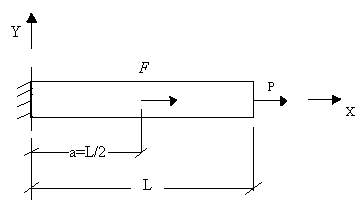
In the example, the bar of Fig. 3.4 is considered:

Figure 4.5

The numerical values of various parameters are as before:

A two-term approximation is chosen for the solution :

(4.8)

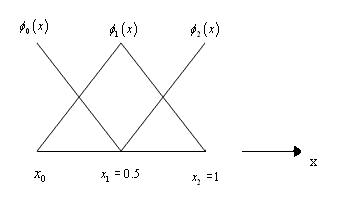
where the functions and are defined as follows :

	for
	for	(4.9)
	for
	for	(4.10)

These functions, along with are shown in Fig. 4.6.

Figure 4.6

Note that the derivatives of the basis functions are given by :

	for
	for	(4.11)
	for
	for	(4.12)

Substituting the expressions (4.11) and (4.12) for and the values of EI and L from equation (4.7) in equation (3.13), the elements of the stiffness matrix [ K ] become :

	(4.13)
	(4.14)
	(4.15)
	(4.16)

Thus

(4.17)

Substituting f = 0 and a = L /2, the expression (3.53) for becomes :

(4.18)

Substituting the values of P , F and L from equation (4.7) and the expressions (4.9) and (4.10) for in the above equation, the elements of the force vector become :

	(4.19)
	(4.20)

Thus,

(4.21)

Thus, the algebraic equations (equation 4.6) become :

(4.22)

The solution of the above equation is:

(4.23)

Then, the approximate solution (equation 4.8) becomes :

	for
	for	(4.24)

This is the same as the exact solution (equation 3.65).

The example in the next section shows that, even for a distributed load, the piecewise linear basis functions can approximate the exact solution to any desired level of accuracy.