Shape Functions

In Lecture 21, the following procedure was adopted for finding the first order Lagrangian shape functions. First, the approximation was expressed as a complete polynomial in ( x , y ) of degree one (eq. 21.1). Then, using the property at , the expressions for shape functions were derived in terms of x and y . For the purpose of numerical integration, this expression was transformed to natural coordinates of the master element. This was done using a linear mapping function (21.10) between the physical element and the master element. This procedure becomes quite cumbersome if the order of approximation is higher . Therefore, we adopt a simpler procedure to obtain the shape functions.

In this procedure, we directly obtain the shape functions in terms of the natural coordinates . The higher order Lagrangian elements are also straight sided elements. Since the mapping is between the straight boundaries of the master element and the straight boundaries of the higher order Lagrangian element, it can be linear. Therefore, we use the same mapping function as before (eq. 21.10). Note that the approximation is a complete polynomial in ( x , y ) of degree p . When the linear mapping function (eq. 21.10) is substituted into it, it becomes a complete polynomial in of degree p .

Note that, in Lecture 21, a complete polynomial of degree p = 1 was used as the approximation and the shape functions turn out to be polynomials of degree one (but not necessarily complete) in the natural coordinates . Similar thing happens for . Thus, each shape function can be assumed as a complete polynomial of degree p in . Since, the approximation is Lagrangian, we can use the property (eq. 21.7)

(23.4)

of the shape functions to determine the coefficients in the polynomial expressions of the shape functions. Thus, the procedure to be adopted for obtaining the shape functions corresponding to the p -th order Lagrangian approximation can be stated as follows :

• First, express each shape function as a complete polynomial of degree p in the natural coordinates .
  
• Next, use the property (eq. 23.4) of the Lagrangian shape functions to determine the coefficients in the polynomial expressions of .
  
• Finally, to make the shape function expressions symmetric, introduce

(23.5)

As an illustration, we demonstrate the procedure for the second order Lagrangian approximation, i.e., p = 2. As stated earlier, the number of various nodes for this element are :

• Number of nodes per element : ,
• Number of boundary nodes : ,
• Number of internal nodes : .

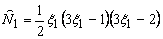
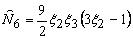
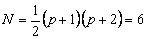
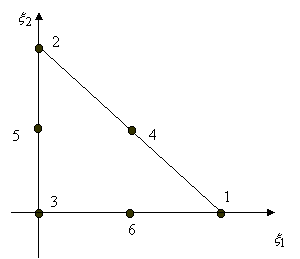
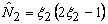
The master element in plane along with the local node numbering scheme is shown in Fig. 23.2.

Figure 23.2 Second Order Lagrangian Triangular (Master) Element.

Out of the 6 nodes, 3 are placed at the vertices. The remaining 3 nodes are placed on the three boundaries. To achieve a proper variation of the primary variable, these nodes should not be too close to the vertices. Instead, they should be closer to the boundary mid-points. In Fig. 23.2, they are placed at the boundary mid-pints. Thus, the values of the nodal coordinates are as shown in Table 23.1.

Table 23.1 Nodal Coordinates of Element of Fig. 23.2

Node No.
1	1	0
2	0	1
3	0	0
4
5	0
6		0

We first find the expression for the third shape function . The first step is to express as a complete 2 nd degree polynomial :

(23.6)

In the second step, we use the property (23.4) to evaluate the coefficients . Thus, the value of is 1 at 3 rd node and 0 at the other nodes. The nodal coordinates are given in Table 23.1. Substituting these values in expression (23.6), we get the following 6 equations for :

,
	(23.7)

Solving these 6 equations, we get the following values of :

	(23.8)

Substituting these values in equation (23.6), the expression for becomes :

(23.9)

As a last step, we introduce as given by eq. (23.5). Then, the expression (23.9) becomes :

(23.10)

Similarly one can obtain the other 5 shape functions. The shape function expressions are :

,  ,
,  ,	(23.11)

We can use the same procedure to obtain the shape functions corresponding to the third order Lagrangian approximation, i.e., p = 3. As stated earlier, the number of various nodes for this element are :

• Number of nodes per element :   ,

• Number of boundary nodes : ,

• Number of internal nodes : .

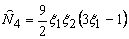
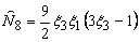
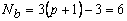
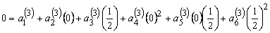
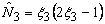
The master element in plane along with the local node numbering scheme is shown in Fig. 23.3.

Figure 23.3 Third Order Lagrangian Triangular (Master) Element

For this element, there is 1 internal node. It (i.e., node no. 10) is placed at the centre. Out of the 9 boundary nodes, 3 are placed at the vertices. The remaining 6 nodes are placed on the three boundaries. For convenience, they are placed such that they trisect the boundary segments. The values of the nodal coordinates are given in Table 23.2.

Table 23.2 Nodal Coordinates of Element of Fig. 23.3

The shape functions for this element can be obtained by the similar procedure. They are given by :

	(23.12)