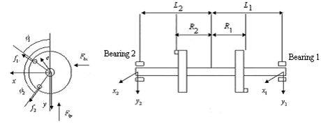
Figure E13.7 A rotor mounted on bearings
Exercise 13.8 For exercise 13.7 use the modal flexible balancing technique. Consider balancing up to second modes. For obtaining the mode shapes the eigen value problem is to be solved.
Exercise 13.10 For a slow speed rotor dynamic balancing, consider a rotor given in Table E13.7. Consider a linearly varying eccentricity with zero centricity at middle of the shaft, and at left and right ends eccentricity of –3μm and – 3μm, respectively. Take discs as the two balancing planes. For numerical simulation two unbalances of 3 gm at 00 and 5 gm at 2400 are considered. The aim would be to obtain these back using simulated responses. Generate responses for a constant speed that is well below (i.e., of the order of 20 Hz) the first critical speed of the shaft at locations 5 cm from either ends of the bearing using the finite element method. Using a trial mass of 4 gm at 400 first in disc 1 and then in disc 2, generate another sets of responses in the same frequency. Obtain various influence coefficients and then estimate back the unbalances of the rotor system at discs 1 and 2. To mimic the actual experimentation different level of random noise (1 to 5 %) may be added to the responses. Two cases may be considered (i) with simply supported end conditions (ii) with hydrodynamic bearing for the data given in Table E13.7.



Interpret physically following cases (i)  (ii)
(ii)  . Obtain an analytical condition (i.e., expression) for which the sense of measurement of phase can also be decided with the help of the fourth measurement.


Exercise 13.14 In a simply supported rotor for flexible rotor balancing, it was found that deflection of the shaft in one of the plane (in a rotating coordinate system) at 35 rad/s could be expressed as

