Exercise Problems
Exercise 13.1 A rotor is being balanced in the cradle-balancing machine by pivoting rotor about a fulcrum (e.g. F1). The following amplitudes of vibrations are observed at the critical speed: (i) 14 μm for the rotor without additional weights, (ii) 10 μm with 5 gm placed in location 0 deg, (iii) 22 μm with 5 gm placed in location 90 deg and (iv) 22 μm with 5 gm placed in location 180 deg. Find the amount and angular location of the necessary correction mass.

Exercise 13.2 A rotor is being balanced in the cradle-balancing machine by pivoting rotor about a fulcrum (e.g. F1). The following amplitudes of vibrations are observed at the critical speed: (i) 10 μm for the rotor without additional weights, (ii) 15 μm with 6 gm placed in location 0 deg., (iii) 20 μm with 6 gm placed in location 90 deg, and (iv) 12 μm with 6 gm placed in location 180 deg. Find the amount and angular location of the necessary correction mass.

Exercise 13.5 For the dynamic balancing of a rotor by using influence coefficients method, if the uncertainty in the measurement of the vibration amplitude and phase are 2 and 5 percent, respectively. Calculate the uncertainty of the magnitude and the phase of influence coefficients and correction masses. Give all the intermediate formulations

Exercise 13.6 Justify your answer for the following cases: a) For the dynamic balancing of a flexible rotor at one particular speed how many minimum numbers of balancing-planes are required? b) For the dynamic balancing of a flexible rotor, in general, how many minimum balancing-planes are required? c) For flexible shaft whether imbalance changes with the shaft speed? d) Apart from balancing the rotor what are the other methods by which the amplitude of the synchronous whirl can be reduced?

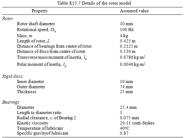
Exercise 13.7 For the balancing of a flexible rotor as shown in Fig. E13.7 and corresponding data given in Table 13.7. Take discs as the two balancing planes. For numerical simulation two unbalances of 3 gm at 00 and 5 gm at 2400 are considered. The aim would be to obtain these using simulated responses. Generate responses with respect to frequency up to above second critical speeds of the shaft at locations 5 cm from either ends of the bearing using the finite element method. Using a trial mass of 4 gm at 400 first in disc 1 and then in disc 2, generate another sets of responses in the same frequency range. Obtain the variation of various influence coefficients with the speed and then estimate back the unbalances of the rotor system at discs 1 and 2. To mimic the actual experimentation different level of random noise (1 to 5 %) may be added to the responses. Two cases may be considered (i) with simply supported end conditions (ii) with hydrodynamic bearing for the data given in Table 13.7.