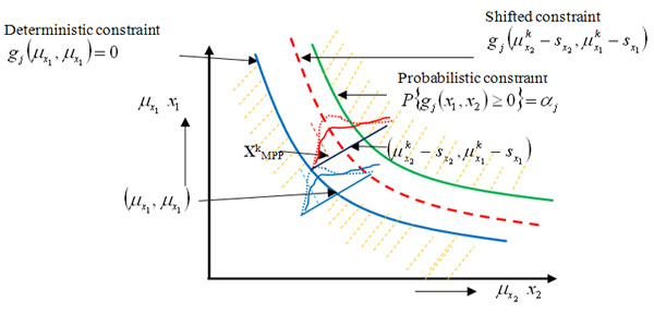
Figure 12.9: Shifting of the constraint boundary

Figure 12.9, corresponds to two different co-ordinate systems, viz (i)  vs  (random space) and (ii) μ₁ vs μ₂ (design variables) and if we do not consider any uncertainty, then g(μ₁, μ₂) = 0 is the constraint boundary in the deterministic design, while for the uncertainty case, the constraint boundary is . The probabilistic constraint feasible region is a reduced region in comparison to the deterministic constraint as the reliability of probabilistic constraint is much higher than that achieved for the deterministic constraint. Determining probabilistic constraint boundary requires reliability analysis, since  is equivalent to g_j(x_MPP, d, p_MPP) = 0, where (x_MPP, p_MPP) is the inverse MPP point and evaluating a probabilistic constraint at (μ₁,μ₂) is equivalent to evaluating the deterministic constraint at the inverse MPP point. The employment of the equivalent deterministic optimization formulation allows us to use an effective single loop strategy and with this strategy, deterministic optimization and reliability assessment are conducted in sequential series. In Figure 12.9, what is also interesting is to note the red and blue (dotted and the continuous) joint distribution functions, , where the bold (dotted) curves signify the non-normal (normal) distributions, such that the corresponding probability of failure and hence the MPP points would definitely dependent on the joint distributions.