Reliability Analysis

To illustrate (12.3) further, let us consider Figure 12.6 (a), in which  is plotted against  and the shaded area underneath the probability density function  depicts the case when this area is greater than or equal to α_j, i.e., , holds true. So logically it implies that given  as the joint distribution function, the shaded area depicts the reliability corresponding to the jth constraint, . To understand this further we discuss the concept of reliability analysis which offers tools for making reliable decisions with the consideration of uncertainty in design variables and/or parameters. Thus in reliability analysis, given a pre-specified performance level, one is interested to find the probability/reliability greater or less than that pre-specified performance. So in order to use (12.3) we need to evaluate the reliabilities of ,  and in presence of these multiple constraints, some of them may never be active and consequently their reliabilities are extremely high (i.e., almost 1.0). Although these constraints are the least critical, the evaluations of these reliabilities will unfortunately dominate the computational effort in probabilistic optimization. The solution to this, is to perform the reliability assessment only up to the necessary level, hence, a formulation of percentile performance (inverse reliability) is used and formulation of the same is as follows, i.e., , where, is the αj-percentile performance of , namely , where it indicates  is exactly equal to the desired reliability α_j. This is illustrated in the Figure 12.6 (b), where the shaded area is again equal to the desired reliability α_j, and  point is called the αj-percentile of function .

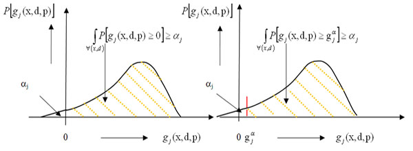
Figure 12.6 (a) & (b): General representation of reliability constraint & αj-percentile reliability constraint