Corresponding Z-transform:
When ![]() = constant, it represents a straight line from the origin at an angle of
= constant, it represents a straight line from the origin at an angle of ![]() rad, measured from positive real axis as shown in Figure 3 (b).
rad, measured from positive real axis as shown in Figure 3 (b).
Constant damping ratio loci: If ![]() denotes the damping ratio:
denotes the damping ratio:
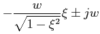 |
|||
![]() is the natural undamped frequency and
is the natural undamped frequency and
![]() . If we take Z-transform
. If we take Z-transform
For a given ![]() or
or ![]() , the locus in s-plane is shown in Figure 4(a).
, the locus in s-plane is shown in Figure 4(a).
In z-plane, the corresponding locus will be a logarithmic spiral as shown in Figure 4(b), except for ![]() or
or ![]() and
and ![]() or
or
![]() .
.
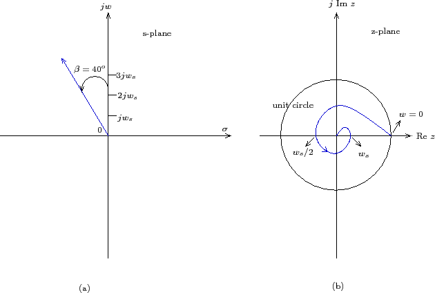
Figure 4: Constant damping ratio locus in (a) s-plane and (b) z-plane