1. Relationship between s-plane and z-plane

In the analysis and design of continuous time control systems, the pole-zero configuration of the transfer function in s-plane is often referred. We know that:

. Left half of s-plane $\Rightarrow$ Stable region.

. Right half of s-plane $\Rightarrow$ Unstable region.

For relative stability again the left half is divided into regions where the closed loop transfer function poles should preferably be located.

Similarly the poles and zeros of a transfer function in z-domain govern the performance characteristics of a digital system.

One of the properties of F*(s) is that it has an infinite number of poles, located periodically with intervals of $\pm mw_{s}$ with m = 0, 1, 2,......, in the s-plane where $w_{s}$ is the sampling frequency in rad/sec.

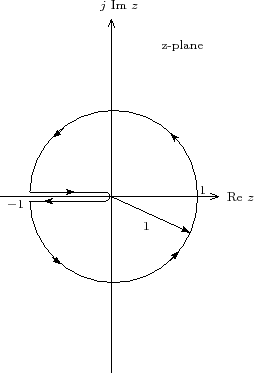
If the primary strip is considered, the path, as shown in Figure 1, will be mapped into a unit circle in the z-plane, centered at the origin.

**Figure 1:** Primary and complementary strips in s-plane
$\begin{figure}\centering \input{m2l2f1.pstex_t}\end{figure}$

The mapping is shown in Figure 2.

**Figure 2:** Mapping of primary strip in z-plane
$\begin{figure}\centering \input{m2l2f1a.pstex_t}\end{figure}$