Since it is difficult to obtain the solution for a nonlinear set of differential equations, we try to utilize a computer program which numerically computes the solution at discrete points in time. An alternative would have been to implement a setup using scaled physical elements which mimic the differential equations, i.e., an analog computer. However, given their flexibility, numerical evaluation using computers is convenient and economical.
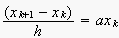
So how do we solve the differential equations numerically ? Let us consider a simple example:

If we wish to obtain the solution denoted by x0, x1, x2, ....xk at the closely spaced time instants t = 0, h, 2h, ....., kh, then we can approximate the above equation as:
Therefore if xk is known, xk+1 can be obtained by
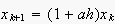
Therefore, if the initial condition x0 is known, we can recursively find the solution of x at discrete instants of time. The approximation is likely to work well only if h is "small enough".
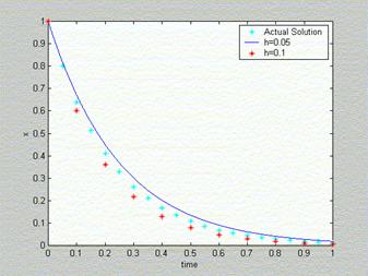
To illustrate this, consider the numerical solution at discrete points and compare it with the correct solution:

Let us take the constant a = -4.
We see from the figure above that the approximation works better for smaller h.
The method that we have presentated is in fact the simplest possible one and is called "Euler's Method" of numerical integration.
|
(click to enlarge)
|
It is not difficult to see that another possible approximation of the differential equation could be:
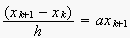
This is called the "Backward Euler" method. The numerical solution obtained using different approximations and different values of h could vary. Inappropriate selection of the method and the time step h can lead to errors which can cause erroneous conclusions. |