Module 7: Nonlinear Finite Element Method Re-Visited
Lectures 31 – 35:
- Concept of Nonlinearity,
- Material Nonlinearity,
- Geometric Nonlinearity,
- Contact Nonlinearity,
- Nonlinear Constitutive relations, Incremental formulation, Solution of Nonlinear Equations
Key-Words: Material Nonlinearity, Geometric Nonlinearity, Contact Nonlinearity, Incremental Formulation, Solution Strategy
Concept of
STRUCTURAL NONLINEARITIES
Introduction
Solution of many engineering problems is based on linear approximations. In structural analyses, these approximations are represented by consideration that
- displacements are small and can be neglected in equilibrium equations,
- the strain is proportional to the stress (linear Hookean material model),
- loads are conservative, independent on displacements,
- supports of the structure remain unchanged during loading.
Consequently, in the Finite Element Analysis (FEA), the constitutive equations describing the structural behavior is then linear
 |
………………..(1) |
where K is the stiffness matrix of the structure, d is the nodal displacements vector and F is the external nodal force vector. Characteristics of solution of this linear problem is that
- the displacements are proportional to the loads,
- the stiffness of the structure is independent on the value of the load level.
In reality, behavior of structures is nonlinear, but divergences from linear response are usually small and may be neglected in most practical problems.
On other hand, solution for many engineering problems needs abandonment of linear approximations. For example, displacements of slender structures (like crane towers, masts etc.) may be so large that changes of the structure shape (or configuration changes) cannot be neglected. Many materials behave nonlinearly or linear material model cannot be used if stress exceeds some value. Moreover, loads may change their orientations according to displacements and supports may change during loading. Consequently, structure behaves nonlinearly. If these phenomena are included in a FEA, the set of equilibrium equations becomes nonlinear and instead of set of linear equations (1) we obtain a set of nonlinear algebraic equations
 |
………………..(2) |
Types of structural nonlinearities
Structural nonlinearities can be specified as
- Geometrical nonlinearities: The effect of large displacements on the overall geometric configuration of the structure.
- Material nonlinearities: Material behavior is nonlinear. Possible material models are:
- nonlinear elastic,
- elastoplastic,
- viscoelastic,
- viscoplastic.
- Boundary nonlinearities, i.e. displacement dependent boundary conditions. The most frequent boundary nonlinearities are encountered in contact problems.
Consequences of nonlinear structural behavior that have to be recognized are:
- The principle of superposition cannot be applied. Thus, for example, the results of several load cases cannot be combined. Results of the nonlinear analysis cannot be scaled.
- Only one load case can be handled at a time.
- The sequence of application of loads (loading history) may be important. Especially, plastic deformations depend on a manner of loading. This is a reason for dividing loads into small increments in nonlinear FE analysis.
- The structural behavior can be markedly non-proportional to the applied load.
- The initial state of stress (e.g. residual stresses from heat treatment, welding, cold forming etc.) may be important.
Concept of time curves
For nonlinear static analysis, the loads are applied in incremental steps using time curves. The “time” variable represents a pseudo time, which denotes the intensity of the applied loads at certain step.
For nonlinear dynamic analysis and nonlinear static analysis with time dependent material properties, “time” represents the real time associated with the loads’ application.
As an example, time curves of forces  and
and  loading simple beam are displayed in Figure- 1. Values of forces at any time are defined as
 |
………………..(3) |
where  and
and  are input values of forces and
  and
and  are load parameters that are functions of time t.
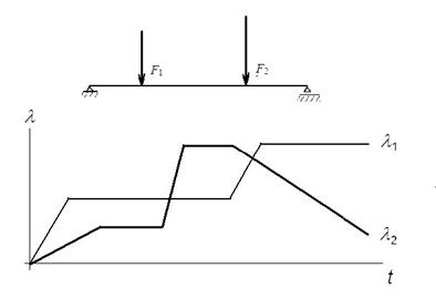
Figure- 1: Example of time curves
The choice of time step size depends on several factors such as the level of nonlinearities of the problem and the solution procedure. Generally, sufficiently small steps are necessary to simulate nonlinear response of a structure with satisfactory accuracy. On the other hand, large number of too small time steps uselessly increases consumption of CPU time. Computer programs are usually equipped with an adaptive automatic stepping algorithm to facilitate the analysis and to reduce the solution time demands.
NONLINEAR FINITE ELEMENT ANALYSIS
Geometric Nonlinearity Concept
Large displacement and small strain behavior
To examine geometrically nonlinear behavior we will start with an example. We assume large displacement, but small rotation and, what is the most important, small strain. The structure is very simple – only one bar truss as is shown in Figure- 2. At the beginning, when the force P is zero, the axial force N in the bar is zero too and bar has its initial length L0.
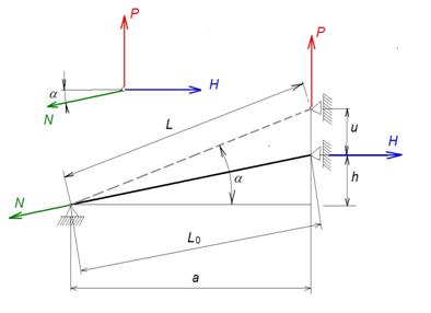
Figure- 2: Example of nonlinear structure – single bar truss
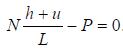
Using the free body diagram shown in Figure- 2, the equilibrium equation is
 |
………………..(4) |
And after substituting 
|
………………..(5) |
Assume that material is linearly elastic with Young’s modulus E. The assumption of small strains means here that changes of the bar cross sectional area A can be neglected. Then axial force in the bar is
|
………………..(6) |
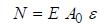
where A0 is the initial cross sectional area and ε is the engineering strain defined as
 |
………………..(7) |
As lengths are given as
 |
………………..(8) |
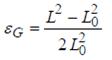
the expression for strain is getting rather complicated. We can overcame this problem by introducing Green’s strain defined as
 |
………………..(9) |
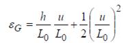
which for our problem becomes
 |
………………..(10) |
Use of this new measure of strain is possible because we can define strain arbitrarily. The only condition is that the strain measure must be objective, which means that is have to be independent on choice of coordinate system and insensitive to a rigid body movement. From equations (7) and (9), it follows that
|
………………..(11) |
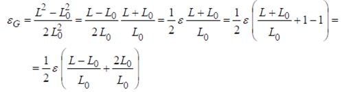
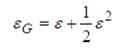
Or
 |
………………..(12) |
Noting that the constitution equation was measured as
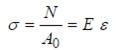 |
………………..(13) |
the same constitutive equation when using Green’s strain should be
|
………………..(14) |
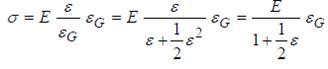
This means that we should use value
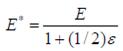 |
………………..(15) |
instead of E in the constitution equation. Fortunately, we can ignore this complication now because for small engineering strain is the difference between engineering and Green’s strain negligible.
For example, consider that  (e.g. mild steel yields at about this value), then
  . This means that difference is only 0,1%, i.e. a value that can be usually neglected. Assuming that strain is small, we can write
  and according to equation (10)
|
………………..(16) |
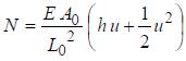
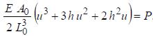
Substituting equation (16) to equilibrium equation (5) and assuming that for small strain is  gives the equilibrium equation
 |
………………..(17) |
Obviously, the equation is nonlinear with respect to displacement u. That means that relation between load P and displacement u is represented not by a straight line as it is when changes of configuration are neglected but by a curve. This nonlinear characteristic for  MPa,
MPa,  mm2, a = 200 mm and h = 20 mm is shown in Figure- 3.
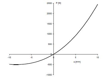
Figure- 3: Geometrically nonlinear behavior of a single bar truss
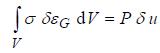
There is another possibility to obtain equation of equilibrium (5) or (17). From principle of virtual displacements, it follows that when the structure is in equilibrium, virtual works of internal and external forces are equal for every kinematic admissible set of virtual displacements. For our structure with one degree of freedom, only one virtual displacement δ u is possible and principle of
virtual displacements has a form
 |
………………..(18) |
where  is virtual strain corresponding to virtual displacement
  . The virtual strain can be expressed from equation (10) as
 |
………………..(19) |
⎟
It is assumed in principle of virtual displacements that virtual displacement is infinitesimal and hence the stress  remains unchanged. Noting that σ and
  are constant over the whole volume V in this case and assuming that changes of the volume can be neglected due to small strain, i.e.
 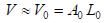 , equation (18) becomes
|
………………..(20) |
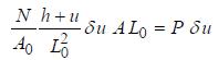
and from this equation it follows that
 |
………………..(21) |
This is the same equation as the equation of equilibrium (5). After substituting for N from (16) the equation (17) will be received again.
Utilization of principle of virtual displacements (PVD) is a convenient way to obtain conditions of equilibrium for complex structures. For general three dimensional case we have three components of displacement u, v, w and six components of Green’s strain
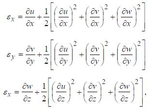 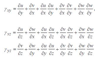 |
………………..(22) |
In finite element method, displacements are interpolated within the finite elements as
 |
………………..(23) |
where  are nodal displacements and Ni are shape functions. Substituting these equations into expressions of Green’s strain components, we obtain
|
………………..(24) |
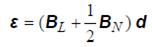
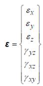
In matrix equation (24)
 |
………………..(25) |
and d is matrix of nodal displacements. Matrix BLis the usual small displacement matrix and matrix BN reflects the fact that Green’s strain is a nonlinear function of displacements. Elements of this matrix are linear functions of nodal displacements d. It might be shown that virtual strain corresponding to the virtual nodal displacements δd is
|
………………..(26) |

According to the principle of virtual displacements, virtual work of internal forces must be equal to virtual work of external forces if the structure is in equilibrium. This is represented by the equation
|
………………..(27) |
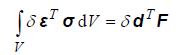
where F is matrix of nodal forces.
We suppose linear relation between stress and strain components, hence
|
………………..(28) |

where D is matrix of material elastic constants.
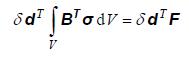
Substituting (26) into (27) gives
 |
………………..(29) |
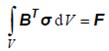
for any kinematic admissible set of virtual displacements δd . Then
 |
………………..(30) |
The last equation is a matrix representation of a set of nonlinear algebraic equations for unknown nodal displacements d.
|
………………..(31) |

Incremental alterative solutions
We have seen that assumption of large displacements leads to nonlinear equation of equilibrium (5) or (17) for a simple bar truss example. Generally, in finite element analysis we have a set of nonlinear equations (31).
Let us start with the bar truss example. The equation of equilibrium (5) or (17) can be written in a form
|
………………..(32) |

where
 |
………………..(33) |
represents a component of internal force.
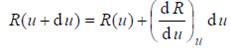
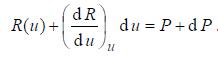
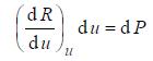
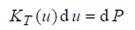
The basic step to solve the nonlinear equation (33) is a linear approximation for small increment of force and corresponding increment of displacement.
Assume that for a prescribed value of force P we managed to find (e.g. by numerical method) a displacement u satisfying the equation (23). Internal force  for new external force
  can be approximated by the linear function
|
………………..(34) |
and approximate condition of equilibrium is
 |
………………..(35) |
Assuming equation (32) gives
|
………………..(36) |
Or
|
………………..(37) |
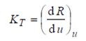
where
 |
………………..(38) |
is called the tangent stiffness. For the particular case of the bar truss, tangent stiffness can be easily found as
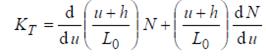 |
………………..(39) |
Using the equation (16) gives
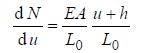 |
………………..(40) |
from which
 |
………………..(41) |
where
|
|
|
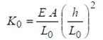 is the linear stiffness
 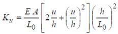 is the initial displacement stiffness
  is the initial stress stiffness.
The linear stiffness, which is independent on displacement, is familiar from small displacement structural analysis. The initial displacement stiffness reflects the effect of displacement on stiffness. The initial stress stiffness reflects the fact that there is an axial force in the bar prior to load increment.
In like manner, we can precede in a general case described by the equation (30) or (31) and derive
 |
………………..(42) |
and
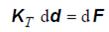 |
………………..(43) |
where
 |
………………..(44) |
is the tangent stiffness matrix. We can also find out that
 |
………………..(45) |
where KT is linear stiffness matrix, K u is initial displacement stiffness matrix and Kσ is initial stress stiffness matrix.
Introduction of tangent stiffness matrix is crucial for solution of nonlinear equations (31). The most widely used methods are briefly introduced in the following text:
Incremental method
The load is divided into a set of small increments ΔFi. Increments of displacements Δdi are calculated from the set of linear simultaneous equations
|
………………..(46) |
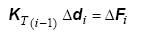
and an updated solution is obtained as
|
………………..(47) |
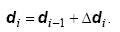
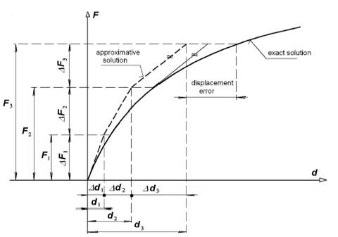
Figure- 4: Incremental method
The procedure is shown in Figure- 4. It is obvious that solution error, i.e. difference from exact solution gradually cumulates. To reduce error, large number of small incremental steps has to be done that is inefficient. On the other hand, division of loading process into sufficiently small increments is necessary to model load path dependent behavior of a structure. Dependence of response on a manner of loading, not only of final values of loads is typical for problems with plastic deformation and with friction. In these problems, incremental method is usually combined with one of following methods.
Newton-Raphson method
Suppose that initial displacements d0 are known. The first guess of nodal displacements for load F is calculated by solving set of linear algebraic equations
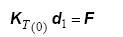 |
………………..(48) |
where
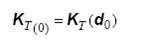 |
………………..(49) |
is tangent stiffness matrix calculated for initial displacements.
As the displacements d1are most probably not accurate, the equilibrium equation (31) is not satisfied and
|
………………..(50) |

that means there are unbalanced (or residual) nodal forces
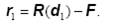 |
………………..(51) |
By computing new tangential stiffness matrix
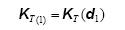 |
………………..(52) |
and solving new set of algebraic linear equations
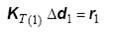 |
………………..(53) |
we will obtain an improved solution
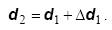 |
………………..(54) |
If  the procedure is repeated until the sufficiently accurate solution is obtained. The iterations are schematically shown in Figure- 5.
This method, known as Newton-Raphson method (NR) is often combined with incremental method as displayed in Figure- 5.
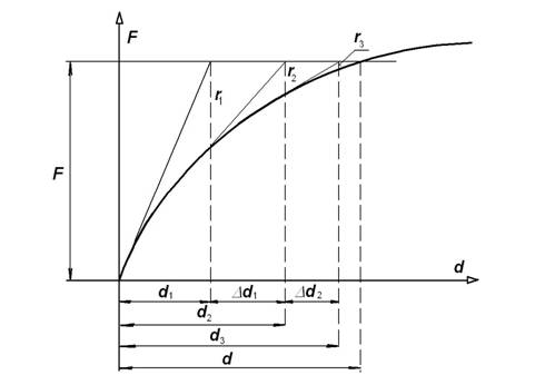
Figure- 5: Standard Newton-Raphson (NR) numerical method
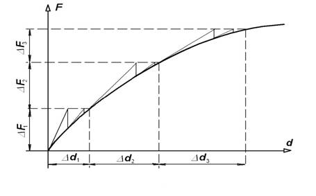
Figure- 6: Combination of Newton-Raphson and incremental methods
Modified Newton-Raphson method
The standard Newton-Raphson method, although effective in many cases, needs the solution of the set of linear equations (53) which is time demanding for large systems. Modified Newton-Raphson method (MNR) differs from standard NR algorithm in that the stiffness matrix is only updated occasionally. In the example shown in Figure- 7, the tangential stiffness matrix is formed and decomposed at the beginning and used throughout the iterations. Advantage of the method is in saving computer time, because factorization of the tangent stiffness matrix is performed only once for the load increment. On the other hand, number of iterations needed is usually large.
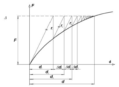
Figure- 7: Modified NewtonRaphson (MNR) method
Quasi-Newton methods
There exist many other methods for solution of the set of nonlinear algebraic equations, so called quasi-Newton methods. The most popular among them is Broyden – Fletcher – Goldfarb – Shanno (BFGS) method.
Linear stability analysis
Theoretically, below a certain critical load a structure is in position of stable equilibrium, whilst above that load the equilibrium may be unstable. Unstable equilibrium means that though the structure is in equilibrium, any arbitrary small disturbance will cause loss of this equilibrium. In many practical problems, the displacements are small for load less than critical and behavior of the structure can be considered as a linear function of applied load. The typical example is Euler strut buckling, Figure- 8.
For axial force N that is less than critical, the strut is in stabile equilibrium. This equilibrium is possible if a lateral load P then deflects the strut as well. If the lateral load is removed, the strut will return to its straight shape.
If the forceN is greater than critical, the strut can remain (theoretically) straight but its equilibrium is unstable, any small lateral load will cause deflection increasing until the collapse.
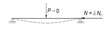
Figure- 8: Buckling of a strut
For load less than critical small longitudinal (in plane) and lateral displacements allow the initial displacement stiffness matrix  to be ignored. The equilibrium equation can be written as
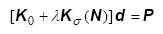 |
………………..(55) |
The elastic critical (buckling) load is given by the lowest value of load parameter λ for which d ≠ 0 when the lateral load  . Physically this means that equilibrium is possible with very small lateral displacements in the absence of any lateral load. In mathematical sense, we have to solve the eigenvalue problem
 |
………………..(56) |
where λ is the eigenvalue and d is the corresponding eigenvector.
It should be noted that due to assumptions accepted the solution represents itself only an estimation of the upper bound of the structure load capacity.
Large displacement and large strain behavior
When strain is large, it is inadmissible to neglect shape and volume changes of a structure. For example, in the simple bar example we have to introduce current cross sectional A instead of initial A0 and current length L instead of initial length L0 in the equations (16) and (17).
Accordingly, integration in the equation (27) expressing the principle of virtual displacements has to be taken over the current volume. This brings problems, as the current volume is unknown, because it depends on displacements that are unknown too and must be calculated first. To solve this problem, it is necessary to introduce a transformation so that integrals are taken over known volume. Two possible ways are briefly described bellow:
Total Lagrangian formulation
In a Total Lagrangian (TL) formulation all integrals are calculated with respect to the initial undeformed configuration of the structure
|
………………..(57) |
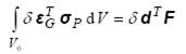
where  is the initial volume. Due to transformation, new measure for stress so called second Piola-Kirchhoff stress tensor
  has to be introduced with Green’s strain tensor
  .
.
Updated Lagrangian formulation
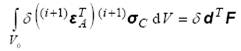
In an Updated Lagrangian (UL) formulation, a known deformed configuration i is taken as an initial state for subsequent configuration (i+1) and this is continually updated as the calculation proceeds
 |
………………..(58) |
In the left side of the equation (2.40),  is Cauchy stress tensor and
  is Almansi strain tensor respectively. Notation
  and
and  means that the strain and stress are in configuration (i+1). Integration is done over volume Vi that is in current configuration i.
Use of different measures for stress and strain in TL and UL formulation follows condition that virtual work of internal forces must be the same irrespective of the volume over which is integration taken1 (1 That means that stress and strain measures must be work conjugate )
MATERIAL NONLINEARITIES
Introduction
Linear elastic FE analysis is based on linear constitutive stress-strain equations
|
………………..(59) |

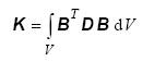
in which the terms of material matrix D are expressed as functions of constant values of modulus of elasticity and Poisson’s ratio. The constant D matrix leads to a constant stiffness matrix K, which is for strain-displacement relationship
|
………………..(60) |

given by
|
………………..(61) |
Departure from linear elasticity implies that the linear elastic constitutive equations are no longer valid, as the material matrix is no longer constant. The non-constant material matrix D represents nonlinear constitutive equations corresponding to the adopted nonlinear material model. Consequently, the conditions of equilibrium derived in FEM from principle of virtual displacements are nonlinear like equations (30) and (31). Solution of these equations is based on the same methods as in geometrically nonlinear case. Usually it is necessary to divide load into increments and perform equilibrium iterations (e.g. by MNR or NR method) for each increment. Moreover, for each load increment there must be performed stress iterations, as the material matrix is function of strain. The strain is unknown a priori and will be computed only.
Material nonlinearities are often combined with geometrical and/or boundary nonlinearities.
Nonlinear elasticity models
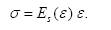
Nonlinear elastic behavior of materials can be formulated in several ways. The simplest is total formulation, where the stress and strains are defined in terms of the secant modulus of elasticity Es, see Figure- 9.
|
………………..(62) |
In hypo-elastic formulation, the relationship between the increments of stress and strain are defined by the tangential modulus of elasticity 
|
………………..(63) |

The nonlinear elastic material law can also be formulated in terms of hyperelastic formulation, which assumes the existence of strain energy density function U and the corresponding complementary energy density function  such
such
|
………………..(64) |
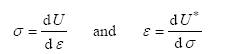
The hyperelastic material model is usually used for rubberlike materials.
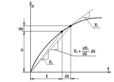
Figure- 9: Nonlinear elasticity model
Material models for multiaxial states of stress are usually based on generalization of linear problem concepts. For example, in a hyperelastic formulation components of stress tensor are computed as
 |
………………..(65) |
that means
 |
………………..(66) |
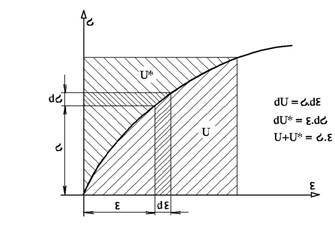
Figure- 10: Strain energy density functions U and 
For any nonlinear elastic material model, it is possible to define relation between stress and strain increments as
|
………………..(66) |
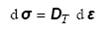
where matrix DT is function of strains ε. Consequently, a set of equilibrium equations we receive in FEM is nonlinear and must be solved by use of any method (e.g. NR) described above.
Elastoplastic material model
Yielding criterion
Experiments indicate that linear elastic model is acceptable only within a limited range of stress. As an example, the stress-strain curve from tension test of steel specimen is shown in Figure- 11. Until the yield stress represented by point A (in the given case  MPa) the deformations are elastic and stress-strain relation may be described as
  . When the stress level exceeds the yield stress, an elasto-plastic constitutive law governs the relationship between increments of stress and strain.
Due to lack of information2, approximate stress-strain curves are usually used in analysis. Bilinear approximation defined by yield stress, modulus of elasticity  and tangential modulus
  is shown in Figure- 12. If
  , material model is elastic-perfectly plastic. If
  material model assumes strain hardening. (2 In a design process, the real material curve is usually unknown, only basic values like yield stress etc. are available. Moreover, the material properties slightly differ by different supplies. )
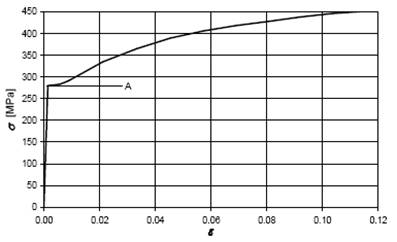
Figure- 11: Typical stress-strain curve for mild steel
It should be noted that curves in Figure-s 11 and 12 are for tensile behavior. It is usually assumed that similar curves for compressive behavior are applicable if there has been no history of plastic deformation.
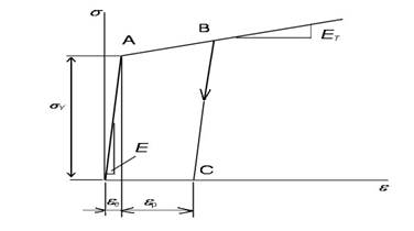
Figure- 12: Elastoplastic model with linear strain hardening
The indication of yielding under multi-axial (more than three axes) conditions in metals is obtained from experiments usually conducted on cylindrical samples subjected to combined axial load and torque. Experiments suggest that there is no significant difference in behavior of metals in tension or compression and no volume change associated with yielding and no effect of mean stress level on yielding can be assumed.
In a mathematical description, onset of yielding may be represented by a scalar function termed the yield function F. The yield function is written in a form, which leads to the conditions
 for elastic and for elastic and  for plastic deformation for plastic deformation |
………..(67) |
In engineering practice, two following conditions for yielding are most frequently used:
- Von Mises yield criterion
|
………………..(68) |

where σ1, σ2 and σ3 are principal stresses. Thus, yield occurs when the effective stress  reaches the yield stress value σy
 |
………………..(69) |
- Tresca yield criterion
|
………………..(70) |

The largest difference between these two classical yield criteria is about 15% for the pure shear stress state. For other stress states is the difference less. Hence, both criteria are frequently considered as equivalent in engineering practice.
Any yield condition that is function of stress tensor components σ and material parameters κ
|
………………..(71) |

defines a yield surface in principal stress space, see Figure- 13. Stress points that lie inside the yield surface are associated with elastic stress states whereas those that lie on the surface represent plastic stress states. No stress point can be outside the yield surface.
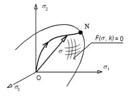
Figure- 13: Yield surface
Post yielding behavior
The fundamental assumption in describing post-yielding behavior is the decomposition of the total strain increment into an elastic (recoverable) part and a plastic (irreversible) part. For uniaxial stress state is, according to Figure- 14.
|
………………..(72) |
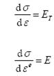
and plastic strain increment is then
|
………………..(73) |
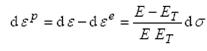
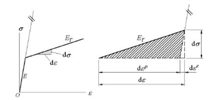
Figure- 14: Decomposition of the total strain increment
By analogy, in multi-axial (other than isotropic cases) stress state the total strains we decompose into elastic and plastic parts too
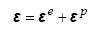 |
………………..(74) |
In multi-axial (other than isotropic cases) cases, subsequent loading after first yield produces further plastic deformation that can result in a modification of the shape and/or position of the yield surface.
For a perfectly plastic material, the yield surface remains unchanged during plastic deformation. For a strain hardening material, plastic deformation produces a change in shape and position of the yield surface. This means that initial yield surface is gradually replaced by the subsequent yield surfaces. A modified yield function is adopted which has a form such as
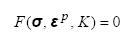 |
………………..(75) |
This yield function depends on the stresses but also the plastic strains and a hardening parameter K. The way in which the plastic strains modify the yield function is defined by hardening rules:
- An isotropic hardening law implies that the yield surface increases in size but maintains its original shape under loading conditions. Schematic representation of isotropic hardening for uniaxial and biaxial stress state is shown in Figure- 15.
- In kinematic hardening, the original yield surface is translated to a new position in stress space with no change of its shape and size as shown in Figure- 16. Kinematic hardening has paramount importance in modelling cyclic behavior.
- The combination of the two principal hardening laws leads to a mixed hardening law, where the initial yield surface both expands and translates as a consequence of plastic flow.
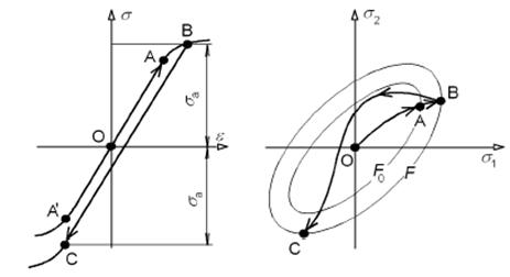
Figure- 15: Isotropic hardening
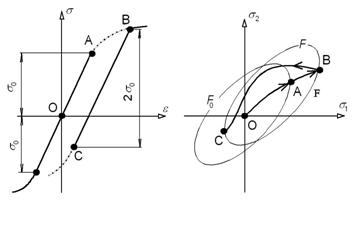
Figure- 16: Kinematic hardening.
Constitutional equations of elasto-plastic material
The yield criterion says whether plastic deformation will occur but says nothing about the plastic behavior of a material after onset of plastic deformations. This is defined by socalled flow rule in which is the rate and the direction of plastic strains is related to the stress state and the stress rate. This relation can be expressed as
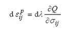 |
………………..(76) |
or in matrix form as
|
………………..(77) |
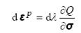
where dλ is a scalar value (to be determined) and Q is a scalar valued function of stress components called plastic potential.
For metals, the called associated flow rule, in which the plastic potential surface coincides with the yield surface, i.e.
 |
………………..(78) |
can be adapted to model plastic flow. For some other materials, non-associated flow rule in which  has to be used to model plastic flow adequately. In the following text we will deal with associated flow rule
|
………………..(79) |
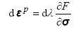
Consider a uniaxial stress state first. The plastic behavior of material is described as
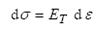 |
………………..(80) |
where  is constant for a bilinear material as obvious from the equations (72) and (73).
In a multi-axial (other than isotropic cases) stress state, we can formulate a similar constitutive equation
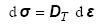 |
………………..(81) |
where tangential material matrix DT can be derived from known stress tensor σ, strain tensor ε and constitutive matrix D from equation (59) in following way:
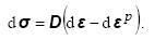
The first step is strain decomposition into elastic  and plastic part
|
………………..(82) |
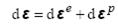
From constitutive law it follows that
|
………………..(83) |

hence
 |
………………..(83) |
From associated plastic flow rule, it follows that
|
………………..(84) |
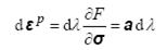
where
|
………………..(85) |

Using equations (83) and (84) we obtain
 |
………………..(86) |
The stress point must lie in yield surface and hence the following consistency conditions must be fulfilled
|
………………..(87) |
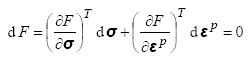
or with respect to equations (83) and (84)
|
………………..(88) |
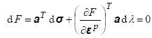
After substituting from equation (86) we obtain
|
………………..(89) |

Or
 |
………………..(90) |
where scalar quantity A is defined as
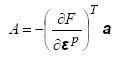 |
………………..(91) |
Now, we can derive parameter dλ from equation (88)
|
………………..(92) |
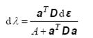
and substituting this expression for dλ into equation (87) we finally obtain
|
………………..(93) |
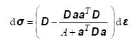
When compare the last equation with equation (81) we can see that
|
………………..(94) |
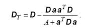
Note that material matrix D is symmetric, i.e. DT = D, hence matrix DT is symmetric as well.
Integration of constitutive equations
We have derived that for infinitesimal increments of stress and strain it holds
|
………………..(95) |

In FE analysis we need to work with finite increments Δσ and Δε for which is the relation above approximate only, so if we use relation
 |
………………..(96) |
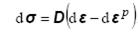
for large increments of stress and strain, an error occurs as stress  in subsequent step will not satisfy constitutive law and consistency condition. Hence, we need to integrate over the increment of pseudo-time
 |
………………..(97) |
where, according to equation (83)
 |
………………..(98) |
It is important to note that if plastic flow is present, the DT changes during increment Δt and as a result, the ratio between total and plastic strain changes too.
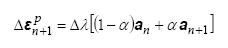
To obtain correct results, various stress increment integration schemes that differ in the degree of approximation have been developed. Frequently used are the following schemes:
Generalized trapezoidal rule
Consider that we know stress  , total strain
  and plastic strain
  at time step n. Then at step n+1
|
………………..(99) |
|||
|
………………..(100) |
|||
|
………………..(101) |
|||


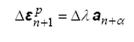
Generalized mid point rule
|
………………..(102) |

|
………………..(103) |
|
………………..(104) |

In both rules, α is a parameter ranging from 0 to 1.
For  we obtain explicit forward Euler integration scheme. Advantage of this algorithm is in its simplicity; disadvantage is that it is conditionally stable only. That means that step increment has to be smaller than some critical value to avoid instability of the solution.
For  we obtain implicit backward Euler integration scheme
|
………………..(105) |
|
………………..(106) |
|
………………..(107) |
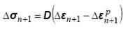
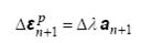

It is obvious that in difference with forward scheme, we deal with values defined at the end of the increment, which are unknown at start of it. Hence, the procedure is of an iterative nature. This means that at beginning of the increment, the trial stress is estimated by assuming elastic deformation and computed values are then checked whether consistency condition and constitutional equation are satisfied. If not, the process is repeated with improved values until the conditions are satisfied.
Numerical procedures
The tangential material matrix DT is used to form a tangential stiffness matrix KT. When the tangential stiffness matrix is defined, the displacement increment is obtained for a known load increment
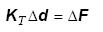 |
………………..(108) |
As load and displacement increments are final, not infinitesimal, displacements obtained by solution of this set of linear algebraic equation will be approximate only. That means, conditions of equilibrium of internal and external nodal forces will not be satisfied and iterative process is necessary. Any of methods mentioned above may be used.
The problem that arises now is the fundamental problem in computational elastoplasticity not only equilibrium equations but also constitutive equations of material must be satisfied. That means that within the each equilibrium iteration step check of stress state and iterations to find elastic and plastic part of strains at every integration point must be included. The iteration process continues until both, equilibrium conditions and constitutive equations are satisfied simultaneously. The converged solution at the end of load increment is then used at the start of new load increment.
Hyperlinks for further detail: