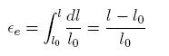
MODULE 2: REVIEW OF SOLID MECHANICS CONCEPTS
Lectures 7 – 10
- Solid-Mechanics 3-D Concepts,
- State-of-stress in three-dimension,
- State of Strain in three dimensions,
- Generalized Hooke’s Law,
- Concept of Plane-stress,
- Concept of Plane-strain,
- Concept of Axi-symmetry,
- Governing-equations in isotropic-elasticity
Key-Words: Stress and Strain in 3-D, 2-D reductions, Constitutive-relations in linear-elasticity
General Introduction
Solid mechanics is the branch of continuum mechanics that studies the behavior of solid materials, especially their motion and deformation under the action of forces, temperature changes, phase changes, and other external or internal agents.
Solid mechanics is fundamental for civil and mechanical engineering, for geology, and for many branches of physics such as materials science. It has specific applications in many other areas, such as understanding the anatomy of living beings, and the design of dental prostheses and surgical implants. One of the most common practical applications of solid mechanics is the Euler-Bernoulli beam equation. Solid mechanics extensively uses tensors to describe stresses, strains, and the relationship between them.
Relationship to continuum mechanics
As shown in the following table, solid mechanics inhabits a central place within continuum mechanics. The field of rheology presents an overlap between solid and fluid mechanics.
Continuum mechanics The study of the physics of continuous materials |
Solid mechanics |
Elasticity |
|
Plasticity |
Rheology |
||
Fluid mechanics |
Non-Newtonian fluids do not undergo strain rates proportional to the applied shear stress. |
||
Newtonian fluids undergo strain rates proportional to the applied shear stress. |
|||
Response models
A material has a rest shape and its shape departs away from the rest shape due to stress. The amount of departure from rest shape is called deformation, the proportion of deformation to original size is called strain. If the applied stress is sufficiently low (or the imposed strain is small enough), almost all solid materials behave in such a way that the strain is directly proportional to the stress; the coefficient of the proportion is called the modulus of elasticity. This region of deformation is known as the linearly elastic region.
It is most common for analysts in solid mechanics to use linear material models, due to ease of computation. However, real materials often exhibit non-linear behavior. As new materials are used and old ones are pushed to their limits, non-linear material models are becoming more common.
There are four basic models that describe how a solid responds to an applied stress:
- Elastically – When an applied stress is removed, the material returns to its undeformed state. Linearly elastic materials, those that deform proportionally to the applied load, can be described by the linear elasticity equations such as Hooke's law.
- Viscoelastically – These are materials that behave elastically, but also have damping: when the stress is applied and removed, work has to be done against the damping effects and is converted in heat within the material resulting in a hysteresis loop in the stress–strain curve. This implies that the material response has time-dependence.
- Plastically – Materials that behave elastically generally do so when the applied stress is less than a yield value. When the stress is greater than the yield stress, the material behaves plastically and does not return to its previous state. That is, deformation that occurs after yield is permanent.
- Thermoelastically - There is coupling of mechanical with thermal responses. In general, thermoelasticity is concerned with elastic solids under conditions that are neither isothermal nor adiabatic. The simplest theory involves the Fourier's law of heat conduction, as opposed to advanced theories with physically more realistic models.
Linear Elasticity
Introduction
The simplest mechanical test consists of placing a standardized specimen with its ends in the grips of a tensile testing machine and then applying load under controlled conditions. Uniaxial loading conditions are thus approximately obtained. A force balance on a small element of the specimen yields the longitudinal (true) stress as
|
………………..(1) |
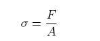
where F is the applied force and A is the (instantaneous) cross sectional area of the specimen. Alternatively, if the initial cross sectional area A0 is used, one obtains the engineering stress
|
………………..(2) |
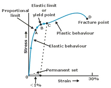
Figure: Strees-strain curve for ductile material
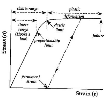
Figure: Strees-strain curve for brittle material
Young's modulus, E, can be calculated by dividing the tensile stress by the extensional strain in the elastic (initial, linear) portion of the stress–strain curve:
|
………………..(3) |
where
E is the Young's modulus (modulus of elasticity) For most materials, this is a large number of the order of 1011 Pa.
F is the force exerted on an object under tension;
A0 is the original cross-sectional area through which the force is applied;
ΔL is the amount by which the length of the object changes;
L0 is the original length of the object.
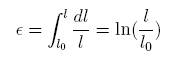
For loading in the elastic regime, for most engineering materials ![]() . Likewise, the true strain is defined as
. Likewise, the true strain is defined as
|
………………..(4) |
while the engineering strain is given by
 |
………………..(5) |
Again, for loading in the elastic regime, for most engineering materials ![]() .
.
Linear elastic behavior in the tension test is well described by Hooke’s law, given by
|
………………..(6) |
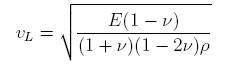
Values of E can be readily determined by measuring the speed of propagation of longitudinal elastic waves in the material. Ultrasonic waves are induced by a piezoelectric device on the surface on the specimen and their rate of propagation accurately measured. The velocity of the longitudinal wave is given by
|
………………..(7) |
Transverse wave propagation rates are also easily measured by ultrasonic techniques and the corresponding relationship is
|
………………..(8) |
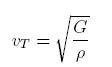
where G is the modulus of elasticity in shear or shear modulus.
The shear modulus is involved in the description of linear elastic behavior under shear loading, as encountered, for instance during torsion testing of thin walled pipes. In this case, if the shear stress is δ and the shear strain γ, Hooke’s law is
|
………………..(9) |
Elements of Linear Elasticity
The aim of continuum mechanics
A rubber band elongates when you pull it. A spring board bends when you stand on it. A bridge vibrates when a truck runs over it. These phenomena show that solids deform. The aim of continuum mechanics is to predict the deformation of a solid in response to a load.
The method of continuum mechanics
The method of continuum mechanics is to view a solid as a continuous distribution of material particles, and predict the deformation of the solid by developing algorithms to calculate the motion of all the material particles.
A solid is made of atoms, each atom is made of electrons, protons and neutrons, and each proton or neutron is made of... This kind of description of matter is too detailed. We will not go very far by thinking of a bridge as a pile of atoms.
Instead, we will develop a continuum theory, in which a solid is modeled by a continuous distribution of material particles. Each material particle consists of many atoms. As time progress, the clouds of electrons deform, and the protons jiggle at a maddeningly high frequency. The material particle represents the collective behavior of many atoms.
At a given time, the material particle occupies a place in a three-dimensional space. The places in the space are labeled by using a system of coordinates. As time progresses, the material particle moves from one place to another place. We can visualize the motion of the material particle by attaching a marker to the particle. Of course we should be careful that the marker should not alter the motion of the material particle. The solid consists of many material particles. Different particles may move in different directions and at different speeds. We can visualize the motion of the entire solid by attaching many markers to the solid.
Displacement:
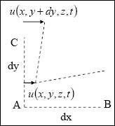
Figure: Strain at a point
At a given time, the positions of all the particles together describe a configuration of the solid. As time progresses, the particles move, and the solid changes its configuration. Any configuration of the solid can be used as a reference configuration. Say we use the configuration of the solid at time t0 as the reference configuration. The configuration of the solid at time t is called the current configuration.
We name a material particle by the coordinates ![]() of the place occupied by the material particle when the solid is in the reference configuration at time
of the place occupied by the material particle when the solid is in the reference configuration at time ![]() . When the solid is in the current configuration at time coordinate t, particle at origin A moves to a new place. The displacement of the particle is the vector by which the particle moves from its place in the reference configuration to its place in the current configuration. At time t, the particle
. When the solid is in the current configuration at time coordinate t, particle at origin A moves to a new place. The displacement of the particle is the vector by which the particle moves from its place in the reference configuration to its place in the current configuration. At time t, the particle ![]() has the displacement
has the displacement ![]() in the x-direction, the displacement
in the x-direction, the displacement ![]() in the y-direction, and the displacement
in the y-direction, and the displacement ![]() in the z-direction.
in the z-direction.
A function of coordinates is known as a field. The field of displacement is a time-dependent field. At a given time, the field of displacement describes the configuration of the solid. Thus, the central aim of continuum mechanics is to develop methods to predict the field of displacement as time progresses.
It is sometimes convenient to write the coordinates of a material particle in the reference configuration as ![]() , and the field of displacement as
, and the field of displacement as ![]() ,
, ![]() .
.
If all the particles in the solid move by the same displacement, the solid as a whole moves by a rigid-body translation. By contrast, if different particles in the solid move by different displacement vectors, the solid deforms. For example, in a bending beam, material particles on one face of the beam move apart from one another (tension), and material particles on the other face of the beam move toward one another (compression). As another example, in a vibrating rod, the displacement varies with the material particle, and the displacement of each material particle is also a function of time.
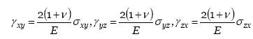
Strain:
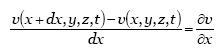
Given a field of displacement in a solid, we can calculate the corresponding field of strain. Consider two material particles of the solid in the reference configuration: particle A at ![]() and particle B at
and particle B at ![]() . In the reference configuration, the two particles are distance dx apart. At a given time coordinate t, the two particles move to new places. The x -component of dy the displacement of particle A is
. In the reference configuration, the two particles are distance dx apart. At a given time coordinate t, the two particles move to new places. The x -component of dy the displacement of particle A is ![]() , and that of particle B is
, and that of particle B is ![]() . Consequently, the distance between the two particles elongates by
. Consequently, the distance between the two particles elongates by ![]() . By definition, the axial strain in the x -direction is
. By definition, the axial strain in the x -direction is
|
………………..(10) |
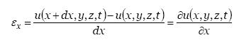
This is a component of strain of the material particle ![]() at time t.
at time t.
The shear strain is defined as follows. Consider two lines of material particles. In the reference configuration, the two lines are perpendicular to each other. The deformation changes the included angle by some amount. This change in the angle defines the shear strain, γ . We now translate this definition into a strain-displacement relation. Consider three material particles A, B, and C. In the reference configuration, their coordinates are ![]() ,
, ![]() , and
, and ![]() . In the deformed configuration, in the x -direction, particle A moves by
. In the deformed configuration, in the x -direction, particle A moves by ![]() and particle C by
and particle C by ![]() . Consequently, the deformation rotates line AC about axis z by an angle
. Consequently, the deformation rotates line AC about axis z by an angle
|
………………..(11) |
Similarly, the deformation rotates line AB about axis z by an angle
|
………………..(12) |
By definition, the shear strain in the xy plane is the net change in the included angle:
|
………………..(13) |
For a solid in a three-dimensional space, the state of strain of a material particle is described by a total of six components. The components of strain relate to the components of displacement as
|
………………..(14) |
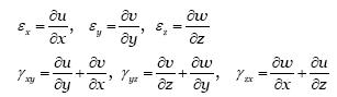
Another definition of the shear strain relates to the definition above by ![]() . With this new definition, we can write the six strain-displacement relations neatly as
. With this new definition, we can write the six strain-displacement relations neatly as
|
………………..(15) |
Stress:
A material particle suffers a state of stress. To talk about stress we need to talk about internal forces. We must expose the internal forces by drawing a free-body diagram. Represent the material particle by a small cube, with its edges parallel to the coordinate axes. Cut the cube out from the body to expose all the internal forces on its 6 faces. Define a component of stress by a component of force per unit area. On each face of the cube, there are three components of stress, one normal to the face (normal stress), and the other two tangential to the face (shear stresses). Now the cube has six faces, so there are a total of 18 components of stress. A few points below get us organized.
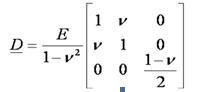
Isotropic linear elastic stress-strain law ![]()
|
………………..(16) |
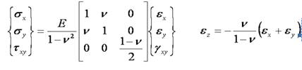
Hence, the ![]() matrix for the for the plane stress case is
matrix for the for the plane stress case is
|
………………..(17) |
|
………………..(18) |
Hence, the ![]() matrix for the for the plane strain case is
matrix for the for the plane strain case is
 |
………………..(19) |
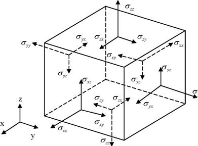
Figure: State at a point
-
Sign convention. On a face whose normal is in the positive direction of a coordinate axis, the component of stress is positive when it points to the positive direction of the axis. On a face whose normal is in the negative direction of a coordinate axis, the component of stress is positive when it points to the negative direction of the axis. If the direct stress is compressive in nature, the sign will be negative and if the direct stress is tensile in nature, the sign will be positive.
-
Equilibrium of the cube. As the size of the cube shrinks, the forces that scale with the volume (gravity, inertia) are negligible. Consequently, the forces acting on the cube faces must be in static equilibrium. Normal components of stress form pairs. Shear components of stress form quadruples. Consequently, only 6 independent components of stress are needed to describe the state of stress of a material particle.
-
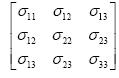
Write the six components of stress in a 3 by 3 symmetric matrix:
|
………………..(20) |
In the above, we have been careless. We have agreed to use ![]() to denote the coordinates of the place in the space occupied by a material particle when the solid is in the reference configuration. But we have then used the same coordinates to denote the place of the material particle in the current configuration when we try to balance force and moment in the current configuration. This practice might be OK when the deformation is small, but will be abandoned later when we do things more rigorously.
to denote the coordinates of the place in the space occupied by a material particle when the solid is in the reference configuration. But we have then used the same coordinates to denote the place of the material particle in the current configuration when we try to balance force and moment in the current configuration. This practice might be OK when the deformation is small, but will be abandoned later when we do things more rigorously.
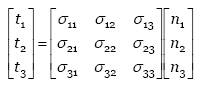
Traction:
Imagine a plane inside a solid. The plane has the unit normal vector n, with three components ![]() . The force per area on the plane is called the traction. The traction is a vector, with three components:
. The force per area on the plane is called the traction. The traction is a vector, with three components:
|
………………..(21) |

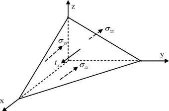
Figure: equilibrium of a tetrahedron
Question: There are infinite many planes through a material particle. How do we determine the traction on each plane?
Answer: You can calculate the traction from
|
………………..(22) |
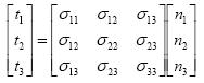
We now see the merit of writing the components of stress as a matrix. Also, the six components are indeed sufficient to characterize a state of stress of a material particle, because the six components allow us to calculate the traction on any plane.
Proof of the stress-traction relation
This traction-stress relation is the consequence of the equilibrium of a tetrahedron formed by the particular plane and the three coordinate planes. Denote the areas of the four triangles by![]() . Recall a relation from geometry:
. Recall a relation from geometry:
|
………………..(23) |
Balance of the forces in the x-direction requires that
|
………………..(24) |
This gives the desired relation
|
………………..(25) |
This relation can be rewritten using the index notation:
|
………………..(26) |
It can be further rewritten using the summation convention:
|
………………..(27) |
Similar relations can be obtained for the other components of the traction vector:
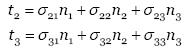
The three equations for the three components of the traction vector can be written collectively in the matrix form, as
 |
………………..(28) |
. Alternatively, they can be written as
|
………………..(29) |
Here the summation is implied for the repeated index j. The above expression represents three equations. We have just described the index notation and summation convention.
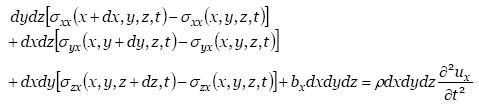
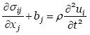
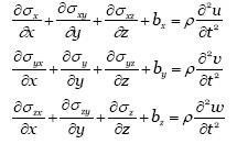
A field of stress:
Imagine again the body in the three-dimensional space. At time t, the material particle ![]() is under a state of stress
is under a state of stress![]() . Denote the distributed external force per unit volume by
. Denote the distributed external force per unit volume by ![]() . An example is the gravitational force,
. An example is the gravitational force, ![]() . The stress and the displacement are time-dependent fields. Each material particle has the acceleration vector
. The stress and the displacement are time-dependent fields. Each material particle has the acceleration vector![]() . Cut a small differential element, of edges dx, dy and dz. Let ρ be the density. The mass of the differential element is
. Cut a small differential element, of edges dx, dy and dz. Let ρ be the density. The mass of the differential element is![]() . Apply Newton’s second law in the x-direction, and we obtain that
. Apply Newton’s second law in the x-direction, and we obtain that
|
………………..(30) |
Divide both sides of the above equation by ![]() , and we obtain that
, and we obtain that
|
………………..(31) |
This is the momentum balance equation in the x-direction.
Similarly, the momentum balance equations in the y-and z-direction are
|
………………..(32) |
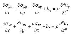
When the body is in equilibrium, we drop the acceleration terms from the above equations. Using the summation convention, we write the three equations of momentum balance as
|
………………..(33) |
Material model- Homogeneity:
When talking about homogeneity, you should think about at least two length scales: a large (macro) length scale, and a small (micro) length scale. A material is said to be homogeneous if the macro-scale of interest is much larger than the scale of microstructures. A fiber-reinforced material is regarded as homogeneous when used as a component of an airplane, but should be thought of as heterogeneous when its fracture mechanism is of interest. Steel is usually thought of as a homogeneous material, but really contains numerous voids, particles and grains.
Material model- Isotropy:
A material is isotropic when response in one direction is the same as in any other direction. Metals and ceramics in polycrystalline form are isotropic at macro-scale, even though their constituents—grains of single crystals—are anisotropic. Wood’s, single crystals, uniaxially fiber reinforced composites are anisotropic materials.
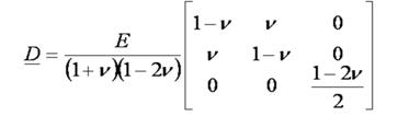
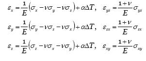
Hooke's law:
For an isotropic, homogeneous solid, only two independent constants are needed to describe its elastic property: Young’s modulus E and Poisson’s ratio u. In addition, a thermal expansion coefficient α characterizes strains due to temperature change. When temperature changes by ∆ T, thermal expansion causes a strain α∆ T in all three directions. The combination of multi-axial stresses and a temperature change causes strains
|
………………..(34) |
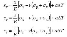
The relations for shear are
|
………………..(35) |
Recall the notation ![]() , and we have
, and we have
|
………………..(36) |
The six stress-strain relation may be written as
|
………………..(37) |
The symbol ![]() stands for 0 when i≠ j and for 1 when i= j. We adopt the convention that a
stands for 0 when i≠ j and for 1 when i= j. We adopt the convention that a
repeated index implies a summation over 1, 2 and 3. Thus, ![]() .
.
Expression stress in terms of strain:
In the above, the 6 components of strain are expressed in terms of the 6 components of stress. From the above relations, we can solve for the components of stress in terms of the components of strain. The resulting relations are![]() ,where µ and λ are known as the Lame constants, given by
,where µ and λ are known as the Lame constants, given by
|
………………..(38) |
List of Equations of Linear Elasticity:
Deformation geometry: strain-displacement relation
 |
………………..(39) |
Stress-traction relation
 |
………………..(40) |
Momentum balance
 |
………………..(41) |
Hooke's Law
 |
………………..(42) |
3-D Elasticity: Equations in other coordinates
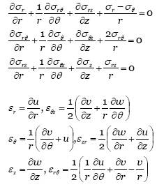
Cylindrical Coordinates (r, θ, z)
u, v, w are the displacement components in the radial, circumferential and axial directions, (r, θ, z) respectively. Inertia terms are neglected.
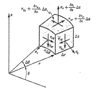
Figure: Cylindrical coordinates (r, θ, z) as commonly used in physics: radial distance r, polar angle θ (theta), and axial distance z. The symbol ρ (rho) is often used instead of r.
|
………………..(43) |
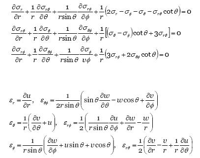
Spherical Coordinates (r, θ ,φ)
θ is measured from the positive z-axis to a radius; φ is measured round the z-axis in a right-
handed sense. u, v, w are the displacements components in the r, θ , φ directions, respectively.
Inertia terms are neglected.
Figure: Spherical coordinates (r, θ, φ) as commonly used in physics: radial distance r, polar angle θ (theta), and azimuthal angle φ (phi). The symbol ρ (rho) is often used instead of r.
 |
………………..(44) |
Stress concentration factor:
Note that the hoop stress is nonzero near the cavity surface, where the hoop stress reaches the maximum. The stress concentration factor is the ratio of the maximum stress over the applied stress. In this case, the stress concentration factor is 3/2.
Stress concentration factors are used in practice to predict failure, and they are listed in handbooks for bodies of many shapes and subject to many types of loads.
Elastic energy:
Consider a rod, initial length L0 and cross-sectional area A0. When a machine applies a force f to the rod, the length of the rod becomes Land the cross-sectional area becomes A. The experimental record gives us the function ![]() , which need not be linear.
, which need not be linear.
When the length of the rod changes from L to ![]() , the machine does work
, the machine does work ![]() to the rod.
to the rod.
We model an elastic solid with an elastic energy, ![]() . This function obeys the following rule. When the length of the rod increases by dL, the increase in the elastic energy of the rod equals the work done by the machine:
. This function obeys the following rule. When the length of the rod increases by dL, the increase in the elastic energy of the rod equals the work done by the machine:
|
………………..(45) |
Define the stress and strain as
|
………………..(46) |
Define the elastic-energy density, w, as the elastic energy per unit volume, namely F
………………..(47) |
Here we have used the initial area and initial length to define the stress, the strain, and the elastic-energy density.
With these definitions, we can rewrite ![]() as
as ![]() . The free energy density is a function of the strain:
. The free energy density is a function of the strain:
|
………………..(48) |
Once we know this function, we can obtain the stress-strain relation by taking the differentiation:
|
………………..(49) |

We next restrict ourselves to small strains, so that we can expand the function ![]() into a Taylor series in the strain:
into a Taylor series in the strain:
………………..(50) |
We will only go up to the quadratic term in strain. The stress is obtained by taking partial differentiation: ![]() .
.
Elastic energy density of a block under shear:
Consider a block, height and ![]() cross-sectional area A0. When a machine applies a shear force f to the block, the block deforms by an shear angle θ. When the angle changes from θ to
cross-sectional area A0. When a machine applies a shear force f to the block, the block deforms by an shear angle θ. When the angle changes from θ to ![]() , the machine does work
, the machine does work ![]() to the block.
to the block.
The elastic energy of the block is a function ![]() . In equilibrium, the change in the elastic energy of the block equals the work done by the machine:
. In equilibrium, the change in the elastic energy of the block equals the work done by the machine:
………………..(51) |
Define the shear stress and the shear strain as
|
………………..(52) |
Define the elastic-energy density, w, as the elastic energy per unit volume, namely F
………………..(53) |
From the above, we have ![]() .
.
The energy per unit volume is a function of the shear strain, w(γ) . Once we know this function, we can obtain the stress-strain relation by taking the differentiation:
|
………………..(54) |
When the block is made of a linearly elastic solid, under shear load, the stress-strain relation is ![]() . Consequently, the energy density function is
. Consequently, the energy density function is
|
………………..(55) |
This result holds only for linear elastic solid in pure shear condition.
When a material particle is in a state of multiaxial stress, the elastic-energy density is a quadratic form of all components of strain. The advantage of using the elastic-energy function becomes clear when the body is in a state of multiaxial stress. We model the elastic solid by stating that the elastic-energy density is a function of all components of strain:
|
………………..(56) |
The components of stress are differential coefficients:
|
………………..(57) |
i.e.,
 |
………………..(58) |
In linear elasticity, we assume that the components of stress are linear in the components of strain. Thus, the energy density is a quadratic form of the components of stain, written as
|
………………..(59) |
Here Cijkl are the components of a fourth-rank tensor called the stiffness tensor. Without losing any generality, we can assume the following symmetries:
|
………………..(60) |
If we count carefully, we should have 21 independent components for a generally anisotropic elastic solid. The components of stress are linear in the components of strain:
.
………………..(61) |
We can also invert this relation to express the strain in terms of the stress:
|
………………..(62) |
Here ![]() components are the components of a fourth-rank tensor called the compliance tensor. They have the same symmetry properties.
components are the components of a fourth-rank tensor called the compliance tensor. They have the same symmetry properties.
Stress-strain relation in a matrix form. We can also write the above equations in another form. The state of strain is specified by the six components:
|
………………..(63) |
In this order we will label them as ![]() .
.
The six components of strain can vary independently. The elastic energy per unit volume is a function of all the six components, ![]() . This is the energy density function.
. This is the energy density function.
When each strain component changes by a small amount, ![]() , the energy density changes by
, the energy density changes by
|
………………..(64) |
Here we use the engineering strains for the shear, rather than the tensor components. We do so to avoid the factor 2 in the above expression. Each stress component is the differential coefficient of the energy density function:
|
………………..(65) |
If the function ![]() is known, we can determine the six stress-strain relations by the differentiations. Consequently, by introducing the elastic-energy function, we only need to specify one function, rather than six functions, to determine the stress-strain relations.
is known, we can determine the six stress-strain relations by the differentiations. Consequently, by introducing the elastic-energy function, we only need to specify one function, rather than six functions, to determine the stress-strain relations.
The above considerations apply to solids with linear or nonlinear stress-strain relations. We now examine linear elastic solids. For the stress components to be linear in the strain components, the energy density function must be a quadratic form of the strain components:
|
……………….(66) |
Here ![]() are 36 constants. The cross terms come in pairs, e.g.,
are 36 constants. The cross terms come in pairs, e.g., ![]() . Only the combination
. Only the combination ![]() will enter into the stress-strain relation, not
will enter into the stress-strain relation, not ![]() and
and ![]() individually. We can call
individually. We can call ![]() by a different name. A convenient way to say that there is only one independent constant is to just let
by a different name. A convenient way to say that there is only one independent constant is to just let ![]() . We can do the same for other pairs, namely,
. We can do the same for other pairs, namely,
|
………………..(67) |
The matrix ![]() is symmetric, with 21 independent elements. Consequently, 21 constants are needed to specify the elasticity of a linear anisotropic elastic solid. Because the elastic energy is positive for any nonzero strain state, the matrix
is symmetric, with 21 independent elements. Consequently, 21 constants are needed to specify the elasticity of a linear anisotropic elastic solid. Because the elastic energy is positive for any nonzero strain state, the matrix ![]() is positive-definite.
is positive-definite.
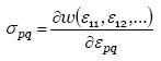
Recall that each stress component is the differential coefficient of the energy density function, ![]() . The stress relation becomes
. The stress relation becomes
………………..(68) |
We list the six components of stress as a column, and list the six components of strain as another column, so that the six stress-strain relations take the form
|
………………..(69) |

The physical significance of the constants ![]() is now evident. For example, when the solid is under a uniaxial strain state,
is now evident. For example, when the solid is under a uniaxial strain state, ![]() , the six stress components on the solid are
, the six stress components on the solid are ![]() . The matrix
. The matrix ![]() is known as the stiffness matrix.
is known as the stiffness matrix.
Inverting the matrix, we express the strain components in terms of the stress components:
 |
………………..(70) |
The matrix ![]() is known as the compliance matrix. The compliance matrix is also symmetric and positive definite.
is known as the compliance matrix. The compliance matrix is also symmetric and positive definite.
The components of the stiffness tensor relate to the corresponding components of the stiffness matrix as
|
………………..(71) |
However, the corresponding relations for compliance are
………………..(72) |
An isotropic, linear elastic solid is characterized by two constants (e.g., Young’s modulus and Poisson’s ratio) to fully specify the stress-strain relation. Some solids are anisotropic, e.g., fiber reinforced composites, single crystals. Each stress component is a function of all six strain components. Consequently, 21 constants are needed to specify the elasticity of a linear anisotropic elastic solid.
A crystal of cubic symmetry:
For a crystal of cubic symmetry, such as silicon and germanium, when the coordinates are along the cube edges, the stress-strain relations are
|
………………..(73) |

The three constants C11, C12 and are independent for a cubic crystal. Isotropic solid is a special case, in which the three constants are related,
|
………………..(74) |
A fiber-reinforced composite: For a fiber reinforced composite, with fibers in the x3 direction, the material is isotropic in the x1 and x2 directions. The material is said to be transversely isotropic. Five independent elastic constants are needed. The stress-strain relations are
|
………………..(75) |

Review of Plane Stress and Plane Strain Elasticity
3D Elasticity Problem
The three dimensional problem of the theory of elasticity (3D elasticity problem) consists of:
- Governing differential equation (equilibrium equations) + boundary conditions
- Strain-displacement relationship (Kinematic equations, Cauchy equations or equations of the geometry)
- Stress-strain relationship (Constitutive equations)
There are some special cases:
- 2D (plane stress, plane strain)
- Axisymmetric body with axisymmetric loading
- Principle of minimum potential energy
This lecture reviews aspects of structural mechanics within the following assumptions:
- Small displacements — equilibrium in the displaced configuration of a structure is adequately represented by the geometry of the original configuration.
- Small strains — second order derivatives of strain have small effect.
- Linear, elastic materials — the material is elastic (all strain energy is recoverable) and the stress is a linear function of strain.
The equations of elasticity relate strain and stress in such a way that equilibrium, compatibility, and the elastic material law are all satisfied. Later in the course we will relax some of these assumptions and consider second-order deformations and, possibly, inelastic materials.
The following figure shows 3D Elasticity Problem definition:
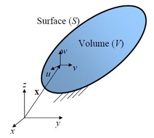
Figure: 3D Elasticity Problem (RVE)
where
V: Volume of body
S: Total surface of the body
The deformation at point ![]() is given by the 3 components of its displacement
is given by the 3 components of its displacement
|
………………..(76) |

We have to note that![]() , i.e., each displacement component is a function of position.
, i.e., each displacement component is a function of position.
Two basic types of external forces act on a body
- Body force (force per unit volume) e.g., weight, inertia, etc
- Surface traction (force per unit surface area) e.g., friction
The body forces are shown in the below Figure:
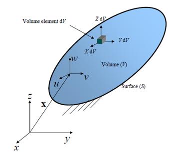
Figure: Body forces on RVE
The forces are as follows:
Body force: distributed force per unit volume (e.g., weight, inertia, etc). It is denoted
 |
………………..(77) |
NOTE: If the body is accelerating, then the inertia force
 |
………………..(78) |
may be considered as a part of g.
The surface traction is shown in the below Figure as:
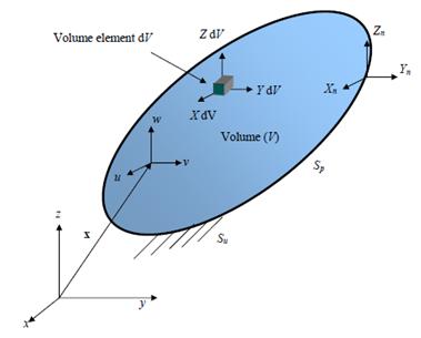
Figure: Surface Traction on RVE
Traction: Distributed force per unit surface area and it is represented by the vector
 |
………………..(79) |
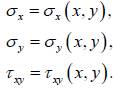
The quantities that describe the stress and strain state of the structure are:
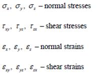 |
………………..(80) |
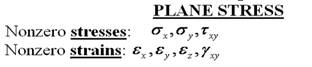
Plane Stress Problem:
Assumptions:
- Let t be the thickness and D be the Diameter of element such that,

- Top and bottom surfaces are free from traction, i. e.,
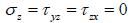
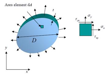
Figure: Plane-Stress problem
Plane stress examples
- Thin plate with a hole
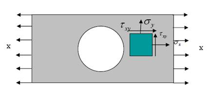
- Thin cantilever plate
The nonzero stresses are:
 |
………………..(81) |
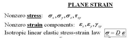
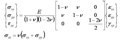
Plane Stain Problem
Assumptions:
- The length of the structure is very large in comparison with the other two dimensions
- The loads are applied only normally to the longitudinal axis (the loads are perpendicular to the z-axis. The loads are uniformly distributed along the length of the body.
- The support conditions are the same along the z-axis
When the structure satisfies the above assumptions all slices has the same stress and strain state. Then, we can write
 |
………………..(82) |
Basic Equations for Plane Stress and Plane Strain
Equilibrium
The equilibrium equation is a differential equation in the deformed configuration. If displacements are small, the equilibrium relationship is valid in the original configuration. More advanced theories define stress tensors for large displacements. Let X, Y are Force components in X-direction and Y-direction respectively.
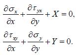 |
………………..(83) |
Kinematic Relationships
The displacements relate the change in geometry from the original to the displaced configuration. Again, we are assuming displacements much smaller than the dimensions of the system. The strain components are defined as
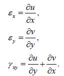 |
………………..(84) |
Constitutive Relationship for Linear Elastic Materials
An elastic material is one in which the stress is a unique function of strain, independent of how the strain is achieved. Another way of saying this is that there is a strain energy function that only depends on the value of the stress and strain tensor. If the stress is a linear function of strain, then Hooke’s law is valid.
We consider homogeneous and isotropic material. For homogeneous material, the properties are the same at any point of the body. For an isotropic material, the properties are the same in any direction. There are two independent elastic constants using the symmetry of an isotropic material. The isotropic constants are:
- E — Young’s modulus of elasticity
- ν — Poisson’s ratio
The strain–displacement relationship for an isotropic material can be written in terms of E, and ν is:
 |
………………..(85) |
where G is a shear modulus.
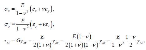
For the plane strain the moduli E and ν should be substituted with the following reduced moduli
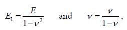 respectively.
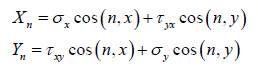
Boundary conditions
The governing equations are complete except for boundary conditions. There are two types of conditions at the boundary of a structure:
Displacement boundary conditions
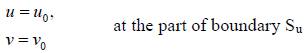
and
Traction boundary conditions
|
………………..(86) |
Each part of the boundary must have a displacement specified or traction in each direction.
Matrix Form of the Governing Equations
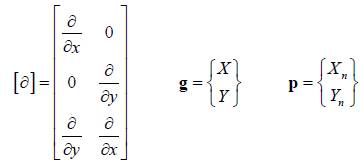
Let us introduce the following vectors and matrices
|
………………..(87) |
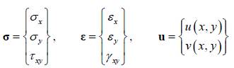
|
………………..(88) |
Additionaly we define initial strain and initial stresses ![]() and
and ![]() .
.
For example initial strain vector due to the temperature variation are
|
………………..(89) |
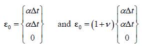
for the plane stress and plane strain, respectively.
We can now write the governing equations in the matrix form as follows:
Equilibrium:
………………..(90) |
Kinematic relationships (Cauchy):
………………..(91) |
Hooke’s law:
………………..(92) |
Displacement boundary conditions
![]()
Force Boundary Conditions:
Hyperlinks for further Details: