Shock Waves
Whenever a stream of traffic flowing under certain stream conditions (say, speed = uA , density = kA, and flow = qA) meets another stream flowing under different conditions (say, speed =uB , density = kB, and flow = qB) a shock wave is started. The shock wave is basically the movement of the point that demarcates the two stream conditions. This demarcation point may move forward or backward or stay at the same place with respect to the road. The rate at which this demarcation point moves (the direction of motion of the vehicles is taken as the positive direction) is referred to as the speed of the shock wave.
In order to see the generation and movement of shock waves consider the distance-time graph shown in Figure 1.
Figure 1
This figure is drawn for the following situation. A slow moving vehicle with speed uB (whose distance-time plot is shown as a dotted line) enters a traffic stream originally moving at uA , kA, qA. This slow moving vehicle slows the traffic and creates another flow condition denoted by uB , kB, qB. From the graph it can be seen that there exists a line (a bold line marked Shock wave 1) that is the locus of the point that demarcates the two flow conditions at any given time. After a while at point Q the slow moving vehicle leaves the traffic stream and the congested condition created by the slow moving vehicle is released, say, at some other stream condition (denoted by uC, kC, qC). Obviously, the point that demarcates the flow conditions uB , kB, qB from the flow conditions uC, kC, qC also causes a shock wave. The locus of this point is marked as Shock wave 2 in the figure. At some time  these two shock waves meet signalling the end of the flow conditions uB , kB, qB. But this time the flow conditions uA , kA, qA meet the flow conditions uC, kC, qC starting Shock wave 3 (see figure 1 ). Interestingly, the vacant area in the figure bounded by the line denoting the motion of last vehicle to go without being caught behind the slow moving vehicle, the dotted line denoting the motion of the slow moving vehicle, and the line denoting the motion of the first vehicle to get released after the departure of the slow moving vehicle, also represent a flow condition; namely the free flow conditions. In the figure this zone is indicated as a stream with conditions u = uf (the free flow speed), k = 0, and q = 0. Hence when the stream condition uB , kB, qB meets the stream condition u = uf , k = 0, and q = 0 a shock wave should and does emanate. The only difference here is that the point which demarcates the two conditions is the same as the point representing the slow moving vehicle; hence, the shock wave that emanates here moves with the slow moving vehicle and the time-distance diagram of this shock wave is the same as the time-distance diagram of the slow moving vehicle. Similarly, the time-distance diagram of the first vehicle that is released is the time-distance diagram of the shock wave that emanates when flow condition uC, kC, qC meets u = uf, k = 0, and q = 0 these two shock waves meet signalling the end of the flow conditions uB , kB, qB. But this time the flow conditions uA , kA, qA meet the flow conditions uC, kC, qC starting Shock wave 3 (see figure 1 ). Interestingly, the vacant area in the figure bounded by the line denoting the motion of last vehicle to go without being caught behind the slow moving vehicle, the dotted line denoting the motion of the slow moving vehicle, and the line denoting the motion of the first vehicle to get released after the departure of the slow moving vehicle, also represent a flow condition; namely the free flow conditions. In the figure this zone is indicated as a stream with conditions u = uf (the free flow speed), k = 0, and q = 0. Hence when the stream condition uB , kB, qB meets the stream condition u = uf , k = 0, and q = 0 a shock wave should and does emanate. The only difference here is that the point which demarcates the two conditions is the same as the point representing the slow moving vehicle; hence, the shock wave that emanates here moves with the slow moving vehicle and the time-distance diagram of this shock wave is the same as the time-distance diagram of the slow moving vehicle. Similarly, the time-distance diagram of the first vehicle that is released is the time-distance diagram of the shock wave that emanates when flow condition uC, kC, qC meets u = uf, k = 0, and q = 0
From the above discussion it is clear that the key parameters of a shock wave are
(i) the point at which it starts,
(ii) the point at which it ends, and
(iii) the speed of the shock wave.
As will be apparent later, of these, the only parameter which needs to be studied in detail is the speed of the shock wave which forms the topic of the next subsection.
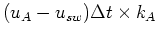
Let a stream flowing under condition A (with uA , kA, and qA) meet another stream flowing under condition B (with uB , kB, and qB). Assume that the speed of the resultant shock wave is  . Then relative to the shock wave vehicles in condition A are moving at a speed of . Then relative to the shock wave vehicles in condition A are moving at a speed of  and those in condition B are moving at a speed of and those in condition B are moving at a speed of  . .
Now, recall that the shock wave is a demarcation between the two conditions. Hence, it can be said that in a time duration of  the number of vehicles crossing over the shock wave from condition A is the number of vehicles crossing over the shock wave from condition A is
 . Similarly, it can be said that in a time duration of the number of vehicles crossing over the shock wave from condition B is . Similarly, it can be said that in a time duration of the number of vehicles crossing over the shock wave from condition B is
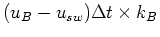 . Note that, physically, some vehicles are crossing over the shock wave from one condition to the other. Since vehicles are neither created nor destroyed in the process of crossing over, the number of vehicles crossing over the shock wave from the perspectives of conditions A and B must be equal. Therefore, . Note that, physically, some vehicles are crossing over the shock wave from one condition to the other. Since vehicles are neither created nor destroyed in the process of crossing over, the number of vehicles crossing over the shock wave from the perspectives of conditions A and B must be equal. Therefore,
Rearranging the terms and substituting  by by  , the following expression can be obtained: , the following expression can be obtained:
It should be noted that the above equation for speed of shock wave can also be obtained using principles of geometry from a distance-time plot of the type shown in Figure 1. Further, the above equation also has a simple graphical interpretation; it states that the speed of the shock wave is given by the slope of the line joining the points representing the two conditions (on a  graph) whose confluence gives rise to the shock wave. Figure 2 shows this graphically. graph) whose confluence gives rise to the shock wave. Figure 2 shows this graphically.
|
Fig. 2: Illustration of the speed of shock waves on a plot. |
There can be three types of shock waves:
(i) the forward moving shock wave, i.e., speed of shock wave is positive (see Figure 3 (a)),
(ii) the stationary shock, i.e., speed of shock wave is zero (see Figure 3 (b)), and
(iii) the backward moving shock wave, i.e., speed of shock wave is negative (see Figure 3 (c)).
Fig. 3: Illustration of different types of shock waves on a plot.
As can be seen from the figure3, the first type of shock wave will occur when a stream with lower flow and lower density meets a stream with higher flow and higher density or when a stream with higher flow and higher density meets a stream with lower flow and lower density. Stationary shock waves will occur when the streams meeting have the same flow value but different densities. The third kind of shock waves will occur when a stream with higher flow and lower density meets a stream with lower flow and higher density or when a stream with lower flow and higher density meets a stream with higher flow and lower density.
In the following web page an example is worked out in order to show how knowledge of shock waves can be used to obtain different traffic flow parameters of interest and also to illustrate how we can obtain information about where a shock wave starts and where it ends (which are the other two parameters related to the description of a shock wave).
|