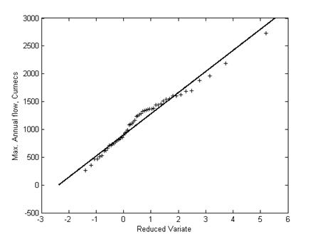
Figure 5.24: Gumbel probability plot for the annual maximum flows in the Tiber River, Italy
Fitting the Gumbel distribution to the annual maximum daily runoff data of a river
Daily runoff data is available for a river for about eighteen years (Table 5.1). If only the maximum runoff data observed in a year is considered for modeling eighteen data points are available. Considering only the maximum runoff also obscures the other relatively larger daily runoffs occurred in any particular year. To avoid this, daily runoffs exceeding 500 Cumecs are considered in this example. This results in a total sample size of 120. This data are used in explaining the Gumbel plotting methodology discussed in the next section.
Table 5.1: Sample calculations involved in Gumbel plotting
S. No. |
Run off |
Plotting position(p), |
Empirical reduced |
Gumbel reduced |
100 |
867.4 |
0.826 |
1.657 |
0.582 |
101 |
871.3 |
0.835 |
1.711 |
0.607 |
102 |
881.1 |
0.843 |
1.767 |
0.669 |
103 |
882.3 |
0.851 |
1.826 |
0.677 |
104 |
902.3 |
0.860 |
1.888 |
0.804 |
105 |
912.7 |
0.868 |
1.953 |
0.871 |
106 |
939.8 |
0.876 |
2.022 |
1.043 |
107 |
947.1 |
0.884 |
2.096 |
1.090 |
108 |
955.1 |
0.893 |
2.175 |
1.141 |
109 |
973.4 |
0.901 |
2.259 |
1.257 |
110 |
992.6 |
0.909 |
2.351 |
1.380 |
111 |
999.6 |
0.917 |
2.450 |
1.424 |
112 |
1006.2 |
0.926 |
2.560 |
1.466 |
113 |
1018.2 |
0.934 |
2.682 |
1.543 |
114 |
1034.2 |
0.942 |
2.820 |
1.645 |
115 |
1073.3 |
0.950 |
2.979 |
1.894 |
116 |
1128.6 |
0.959 |
3.165 |
2.246 |
117 |
1138 |
0.967 |
3.393 |
2.306 |
118 |
1307.2 |
0.975 |
3.685 |
3.383 |
119 |
1506.2 |
0.983 |
4.094 |
4.651 |
120 |
1528.6 |
0.992 |
4.792 |
4.794 |
Gumbel Probability plotting
Two important steps in the Gumbel probability plotting are finding the plotting positions and the reduced variates. Plotting positions are distributed in between zero and one and each plotting position is equally likely to appear. To obtain the plotting positions the data is arranged in the ascending order and the ranks are given from the smallest to the largest variate. In finding the plotting position corresponding to any ordered statistic the rank value of that variate and the rank of the maxima is used. For example, the plotting position corresponding to the 100th ordered statistic is 100/(120+0.3). Sample calculations are shown in the above Table. The parameters used in getting the theoretical reduced variates are: location parameter is 776, scale parameter is 157. Figure 5.24 shows the probability plot of the maximum runoff data of Tiber river, Italy.
Summary
Because the world around is not perfectly reproducible, an understanding of the observation and measurement issues, working knowledge of the theories of probability is necessary to understand the variability. The work of the analyst can be simplified when the problem at hand fits the specifications of one of these common distributions. In this Chapter various observed data have been assumed to follow different discrete and continuous distributions. But, it is necessary to know whether these assumptions are correct or not. For verifying this it is necessary to understand statistics and their distributions that are discussed in forthcoming chapters. In the chapter ‘Hypotheses testing’ the truthfulness of the assumptions is tested.