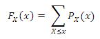
Consider a random variable X defined by the number of heads obtained when two balanced or true coins are tossed, the possible values of X are 0, 1, 2. The resulting probability distribution is described in Table 3.2. The same is shown in the graphical form in Figure 3.1.

Table 3.2: probability distribution function associated to the experiment “tossing two true coins”

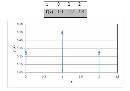
Figure 3.1: Probability mass function for the data given in Table 3.2

Cumulative distribution function for a discrete random variable

Cumulative distribution function (cdf ) of any random variable is denoted by F_X(x). This is also denoted by the probability of the random variable X taking the values that are smaller than or equals to x , P( X ≤ x ). This is a monotonically increasing function bounded in between 0 and 1.

For discrete random variable X,

Cumulative distribution function for the data on experiment "tossing the coin twice", given in table 3.2, is plotted in Figure 3.2.

Another example for the discrete random variables is the number of vehicles crossing a particular location of the road stretch in a given time interval. If the time interval is 1 minute and the road is a single lane road, the possible integer values taken by the discrete random variable may fall in between 1 to 30. Sometimes the number of vehicles arrived in consecutive time intervals may not depend on each other and sometimes may depend on one another. Another example is on a particular day whether it rains or not. In this case the random variable is binary, i.e. it takes either 0 or 1. These examples are explained in detail in the following sections.

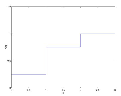
Figure 3.2: Cumulative distribution function of a discrete random variable